Sea ice

Description

The Sea Ice diagnostic is a set of tools to compute and plot time series, seasonal cycles and 2D spatial maps of sea ice metrics. The diagnostic supports analysis of sea ice extent, volume, fraction, and thickness. Time series and seasonal cycles can be computed over a specific region of the Northern or Southern Hemisphere. Default regions are the Arctic and the Antarctic regions, but it is possible to select other regions and custom regions can be defined in the configuration file.

Classes

There is one class that process and analyse the sea ice data, allowing to save the result as NetCDF files:

SeaIce: a class that computes the sea ice extent, volume, fraction, and thickness metrics. The class handles data retrieval, regional selection, integration, and statistical analysis internally for a single model or reference data. It supports time series analysis and seasonal cycle computation with optional standard deviation calculations.
- The methods supported for time series analysis which computes the integrated values over specified regions are:
  - extent: computes the area of ocean cells with at least 15% sea ice concentration (the threshold can be tuned in the configuration file).
  - volume: computes the integrated sea ice thickness.
- The methods supported for 2D spatial analysis, which computes the 2D monthly climatology maps over specified regions are:
  - fraction: produces the 2D monthly climatology maps of sea ice fraction (0-1).
  - thickness: produces the 2D monthly climatology maps of sea ice thickness (meters).

There are other two classes to produce the plots, which support a comparison between multiple models against a reference dataset. These classes can accept a xarray.DataArray, a xarray.Dataset, or a list of xarray.Dataset with a collection of sea ice variables defined per region and calculation method.

PlotSeaIce: a class that produces time series and seasonal cycle plots.
Plot2DSeaIce: a class that produces the plots for the 2D spatial maps and biases for climatological maps over the months.

Note

The extent and volume methods produce time series data, while fraction and thickness methods is associated to 2D spatial maps.

File structure

The diagnostic is located in the src/aqua_diagnostics/seaice directory, which contains both the source code and the command line interface (CLI) script cli_seaice.py.
The default configuration file is located in config/diagnostics/seaice/config_seaice.yaml.
The regional definitions are defined in config/diagnostics/seaice/definitions/regions.yaml.
Notebooks are available in notebooks/diagnostics/seaice directory and contain examples of how to use the diagnostic.

Input variables and datasets

The classes support the following variables, although the Fixer class can convert the acceptable different variable names into the following accepted variables:

siconc (sea ice concentration, GRIB parameter id 31)
sithick (sea ice thickness, GRIB parameter id 32)
sivol (sea ice volume, GRIB parameter id 33)

The diagnostic supports comparison with reference datasets, with OSI-SAF being the default observational reference for sea ice concentration. Custom reference datasets can be configured through the configuration file.

Basic usage

The basic usage of this diagnostic is explained with a working example in the notebook provided in the notebooks/diagnostics/seaice directory. A basic structure of the analysis is the following:

For Time Series Analysis:

from aqua.diagnostics import SeaIce, PlotSeaIce

# Compute sea ice extent (time series calculation)
si = SeaIce(model='IFS-NEMO', exp='historical-1990', source='lra-r100-monthly', loglevel="DEBUG")
result = si.compute_seaice(method='extent', var='siconc')

# Plot time series
psi = PlotSeaIce(monthly_models=result, loglevel='DEBUG')
psi.plot_seaice(plot_type='timeseries', save_pdf=True, save_png=True)

For 2D Spatial Analysis:

from aqua.diagnostics import SeaIce, Plot2DSeaIce

# Compute sea ice fraction (2D maps calculation)
si = SeaIce(model='IFS-NEMO', exp='historical-1990', source='lra-r100-monthly', loglevel="DEBUG")
result = si.compute_seaice(method='fraction', var='siconc', stat='mean', freq='monthly')

# Plot 2D maps
psi_2d = Plot2DSeaIce(models=result, loglevel='DEBUG')
psi_2d.plot_2d_seaice(plot_type='var', method='fraction', months=[3,9],
                      projkw={'projname': 'orthographic'}, save_pdf=True, save_png=True)

Note

The user can also define the start and end date of the analysis and the reference dataset. If not specified otherwise, plots will be saved in PNG and PDF format in the current working directory.

CLI usage

The diagnostic can be run from the command line interface (CLI) by running the following command:

cd $AQUA/src/aqua_diagnostics/seaice
python cli_seaice.py --config <path_to_config_file>

Additionally, the CLI can be run with the following optional arguments:

--config, -c: Path to the configuration file. Default is config/diagnostics/seaice/config_seaice.yaml in the AQUA root directory.
--nworkers, -n: Number of workers to use for parallel processing.
--cluster: Cluster to use for parallel processing. By default a local cluster is used.
--loglevel, -l: Logging level. Default is WARNING.
--catalog: Catalog to use for the analysis. Can be defined in the config file.
--model: Model to analyse. Can be defined in the config file.
--exp: Experiment to analyse. Can be defined in the config file.
--source: Source to analyse. Can be defined in the config file.
--outputdir: Output directory for the plots.
--proj: Projection type for 2D plots. Choices are ‘orthographic’ or ‘azimuthal_equidistant’. Default is ‘orthographic’.

Config file structure

The configuration file is a YAML file that contains the details on the dataset to analyse or use as reference, the output directory and the diagnostic settings. Most of the settings are common to all the diagnostics (see Diagnostics configuration files). Here we describe only the specific settings for the sea ice diagnostic.

The sea ice configuration file is organized into several main sections

Dataset Configuration:

datasets:
  - catalog: null              # mandatory as null
    model: 'IFS-NEMO'          # mandatory
    exp: 'historical-1990'     # mandatory
    source: 'lra-r100-monthly' # mandatory
    regrid: null               # if the diagnostic supports it

Reference Datasets:

references:
  # ---- Extent in NH ----
  - &ref_osi_nh
    catalog: 'obs'             # mandatory
    model: 'OSI-SAF'           # mandatory
    exp: 'osi-450'             # mandatory
    source: 'nh-monthly'       # mandatory
    regrid: 'r100'
    domain: "nh"

The reference datasets are defined using YAML anchors (&ref_osi_nh) and can be reused across different diagnostic blocks. Each reference dataset specifies:

catalog: Data catalog identifier
model: Reference model name (e.g., OSI-SAF, PSC)
exp: Experiment identifier
source: Data source specification
regrid: Regridding target resolution
domain: Geographic domain (nh=Northern Hemisphere, sh=Southern Hemisphere)

Diagnostic Blocks:

Each diagnostic block in CLI config_seaice.yaml:

seaice_timeseries
seaice_seasonal_cycle
seaice_2d_bias

contains the following parameters such as:

seaice_timeseries:
  run: true
  methods: ["extent", "volume"]   # Methods to compute
  regions: ['arctic','antarctic'] # Regions to analyze
  startdate: '1991-01-01'         # Analysis start date
  enddate: '2000-01-01'           # Analysis end date
  calc_ref_std: true              # Calculate reference standard deviation
  ref_std_freq: 'monthly'         # Standard deviation frequency
  varname:                        # Variable mapping for each method
    extent: 'siconc'
    volume: 'sithick'
    fraction: 'siconc'
    thickness: 'sithick'

Method-specific variable mapping:

extent and fraction: Use siconc as variable name (sea ice concentration)
volume and thickness: Use sithick as variable name (sea ice thickness)

Reference dataset assignment:

Each diagnostic block includes a references section that assigns specific reference datasets to methods:

references:
  - <<: *ref_osi_nh
    use_for_method: "extent"    # Use this reference for extent analysis
    varname: "siconc"
  - <<: *ref_psc_nh
    use_for_method: "volume"    # Use this reference for volume analysis
    varname: "sithick"

2D Bias Configuration: The seaice_2d_bias block includes additional parameters for spatial analysis:

seaice_2d_bias:
  months: [3, 9]                # Months to plot (March and September)
  projections:                  # Map projection options
    orthographic:
      projname: "orthographic"
      projpars:
        central_longitude: 0.0
        central_latitude: "max_lat_signed"
    extent_regions:             # Geographic extent for each region
      Arctic: [-180, 180, 50, 90]
      Antarctic: [-180, 180, -50, -90]

projections can be tuned to the user according to the section ‘Projections and custom maps’ in Graphic tools.

Output Configuration:

output:
  outputdir: "./"               # Output directory
  rebuild: true                 # Overwrite existing files
  save_netcdf: true             # Save NetCDF files
  save_pdf: true                # Save PDF plots
  save_png: true                # Save PNG plots
  dpi: 300                      # Plot resolution

Note

The configuration file uses YAML anchors (&ref_osi_nh) and references (<<: *ref_osi_nh) to avoid duplication. This allows the same reference dataset definition to be reused across different diagnostic blocks with method-specific assignments.

CLI processing

The CLI uses separate diagnostic blocks for different types of analysis:

seaice_timeseries: for time series analysis of extent and volume
seaice_seasonal_cycle: for seasonal cycle analysis of extent and volume
seaice_2d_bias: for 2D spatial analysis of fraction and thickness biases

The input parameters can be overridden during the CLI call.

Outputs

After the analysis and processing of the data, the diagnostic can produce the following outputs:

NetCDF files: Time series, seasonal cycle or 2D spatial climatology maps saved in NetCDF format for further analysis.

All plots can be performed and then saved in both PDF and PNG formats with comprehensive metadata describing the plot:

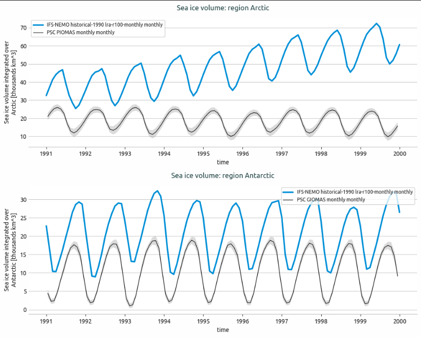
Time series plots: Monthly time series of sea ice extent and volume for specified regions.
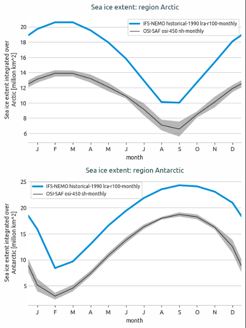
Seasonal cycle plots: Monthly climatology of sea ice metrics with optional standard deviation bands.
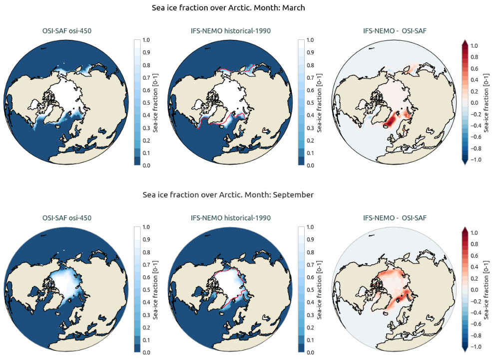
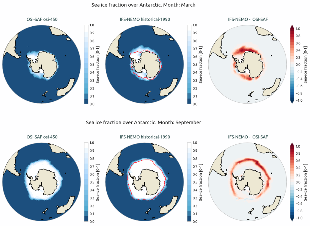
2D spatial maps: Climatological maps of sea ice fraction and thickness for specific months and regions.
Bias maps: Spatial differences between model and reference sea ice data for specific months and regions.

Example Plot(s)

../_images/seaice_ts_volume_Arctic_Antarctic.png

../_images/seaice_seasonalcycle_extent_Arctic_Antarctic.png

../_images/seaice_2d_fraction_Arctic_3-9.png

../_images/seaice_2d_fraction_Antarctic_3-9.png

../_images/seaice_2d_thickness_Arctic_3-9.png

../_images/seaice_2d_thickness_Antarctic_3-9.png

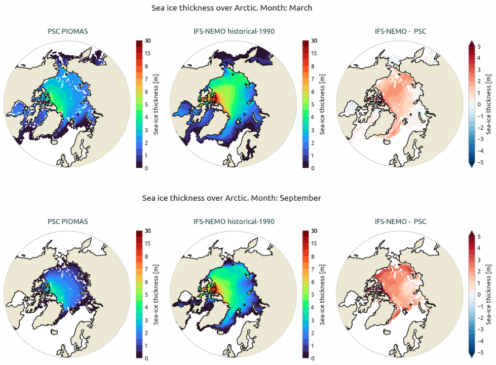
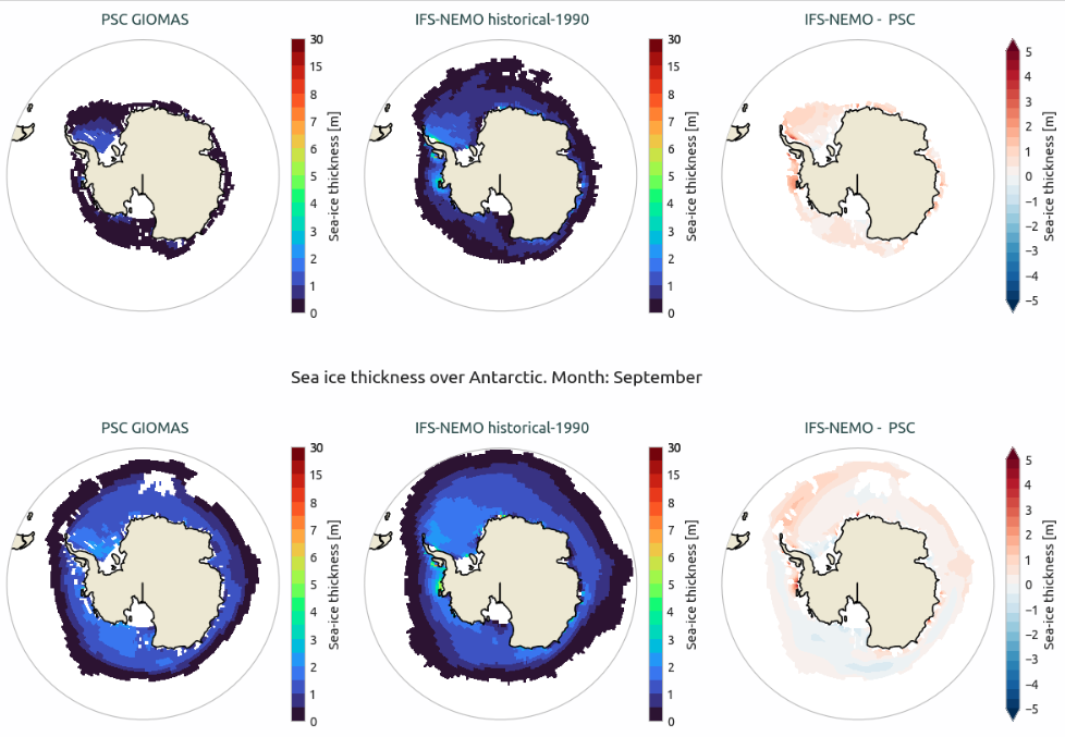
Observations (Reference data)

Default model is IFS-NEMO, experiment is historical-1990, source is lra-r100-monthly.

Details on the reference datasets, are available on the website of the Ocean and Sea Ice Satellite Application Facility (OSI-SAF) here. An updated version of the reference datasets is available in AQUA obs catalog named exp=osi-saf-aqua, which concatentes OSI-SAF osi-450-a1 (1979 - 2021) and OSI-SAF osi-430 (2022 - 2024) datasets.

Available demo notebooks

Notebooks are stored in diagnostics/seaice/notebooks

Authors and contributors

This diagnostic is maintained by Emanuele Tovazzi (@tovaz92, emanueletovazzi [at] cnr.it), member of the AQUA team. Contributions are welcome — please open an issue or a pull request. For questions or suggestions, contact the AQUA team or the maintainers.

Detailed API

This section provides a detailed reference for the Application Programming Interface (API) of the Seaice diagnostic, produced from the diagnostic function docstrings.

class aqua.diagnostics.seaice.Plot2DSeaIce(ref=None, models=None, regions_to_plot: list = ['Arctic', 'Antarctic'], outputdir='./', rebuild=True, dpi=300, loglevel='WARNING')

Bases: object

A class for processing and visualizing surface maps and biases of sea ice fraction or thickness.

Parameters:

ref (xarray.DataArray or xarray.Dataset) – Reference sea ice data.
models (list of xarray.DataArray or xarray.Dataset) – List of models with sea ice data.
regions_to_plot (list) – List of strings with the region names to plot which must match the ‘AQUA_region’ attribute in the data provided as input.
outputdir (str) – Output directory for saving plots.
rebuild (bool) – Whether to rebuild the plots if they already exist.
dpi (int) – Dots per inch for the saved figures.
loglevel (str) – Logging level for the logger. Default is ‘WARNING’.

plot_2d_seaice(plot_type='var', months=[3, 9], method='fraction', projkw=None, plot_ref_contour=False, save_pdf=True, save_png=True, **kwargs)

Plot sea ice data and biases.

Parameters:

plot_type (str) – Type of plot to generate [‘var’ or ‘bias’].
months (list) – List of months to plot, e.g. [2, 9] for February and September.
projkw (dict) – Dictionary with projection parameters for the plot.
save_pdf (bool) – Whether to save the plot as a PDF.
save_png (bool) – Whether to save the plot as a PNG.
plot_ref_contour (bool) – Whether to add a reference line at 0.2 for sea ice fraction.
**kwargs – Additional keyword arguments for customization. See below functions for details.

class aqua.diagnostics.seaice.PlotSeaIce(monthly_models=None, annual_models=None, monthly_ref=None, annual_ref=None, monthly_std_ref: str = None, annual_std_ref: str = None, model: str = None, exp: str = None, source: str = None, catalog: str = None, regions_to_plot: list = ['Arctic', 'Antarctic'], outputdir='./', rebuild=True, filename_keys=None, dpi=300, loglevel='WARNING')

Bases: object

A class for processing and visualizing timeseries of integrated sea ice extent or volume. It is designed to work with AQUA-computed outputs (from the SeaIce diagnostic) repacking them into a unified format for easy comparison, labeling, and plotting.

Parameters:

monthly_models (xr.Dataset | list[xr.Dataset] | None, optional) – Monthly model datasets to be processed. Defaults to None.
annual_models (xr.Dataset | list[xr.Dataset] | None, optional) – Annual model datasets to be processed. Defaults to None.
monthly_ref (xr.Dataset | list[xr.Dataset] | None, optional) – Monthly reference datasets for comparison. Defaults to None.
annual_ref (xr.Dataset | list[xr.Dataset] | None, optional) – Annual reference datasets for comparison. Defaults to None.
monthly_std_ref (str, optional) – Monthly standard deviation reference dataset identifier. Defaults to None.
annual_std_ref (str, optional) – Annual standard deviation reference dataset identifier. Defaults to None.
model (str, optional) – Name of the model associated with the dataset. Defaults to None.
exp (str, optional) – Experiment name related to the dataset. Defaults to None.
source (str, optional) – Source of the dataset. Defaults to None.
catalog (str, optional) – Catalog name of the dataset. Defaults to None.
regions_to_plot (list, optional) – List of region names to be plotted (e.g., [‘arctic’, ‘antarctic’]). If None, all available regions are plotted. Defaults to None.
outputdir (str, optional) – Directory to save output plots. Defaults to ‘./’.
rebuild (bool, optional) – Whether to rebuild (overwrite) figure outputs if they already exist. Defaults to True.
exists. ((overwrite) figure outputs if) – List of keys to include in the output filenames. If None, all keys are included. Defaults to None.
dpi (int, optional) – Resolution of saved figures (dots per inch). Defaults to 300.
loglevel (str, optional) – Logging level for debugging and information messages. Defaults to ‘WARNING’.

plot_seaice(plot_type='timeseries', save_pdf=True, save_png=True, style=None, **kwargs)

Plot sea ice data for each region, either as timeseries or seasonal cycle.

Parameters:

plot_type (str, optional) – Type of plot to generate. Options are ‘timeseries’ or ‘seasonal_cycle’. Defaults to ‘timeseries’.
save_pdf (bool, optional) – Whether to save the figure as a PDF. Defaults to True.
save_png (bool, optional) – Whether to save the figure as a PNG. Defaults to True.
style (str, optional) – Override the plotting style. Default to None (which will get the style from config file or fallback to’aqua’).
**kwargs – Additional keyword arguments passed to the region-specific plotting function.

regions_type_plotter(region_dict, style, **kwargs)

Loops over each region in region_dict and plots data either as a timeseries or a seasonal cycle depending on plot_type attribute.

Parameters:

region_dict (dict) – Dictionary of regions and their associated data.
style (str) – Graphic style of the plot.
**kwargs (dict) – Additional keyword arguments passed on to the underlying plotting function.

Returns:

tuple. The figure and axes objects.

Return type:

(fig, axes)

repack_datasetlists(**kwargs) → dict

Repack input datasets into a nested dictionary organized by method and region. The output dictionary is structured as:

{ method: { region: { str_data: [list of data arrays] }}}

where: ‘method’ is extracted from the dataset attributes (defaulting to “Unknown”). ‘region’ is determined by self._get_region(dataset, data_var). ‘str_data’ is the keyword with the data in input, and each value is a list of data arrays corresponding to that keyword.

Parameters:: **kwargs (dict) – Keyword arguments, where each str_data is linked to the kwargs in plot_timeseries() and each value is a list of xr.Dataset objects.
Returns:: A nested dict containing the repacked data arrays.
Return type:: dict

save_fig(fig, save_png: bool, save_pdf: bool, metadata: dict = None, region_dict: dict = None)

Save a matplotlib figure in PNG and/or PDF format with associated metadata.

Parameters:

fig (matplotlib.figure.Figure) – The figure object to be saved.
save_png (bool) – Whether to save the figure as a PNG file.
save_pdf (bool) – Whether to save the figure as a PDF file.
metadata (dict, optional) – Metadata such as description to be saved. Defaults to None.
region_dict (dict, optional) – Dictionary of regions plotted. Used to generate output filename. Defaults to None.

class aqua.diagnostics.seaice.SeaIce(model: str, exp: str, source: str, catalog=None, regrid=None, startdate=None, enddate=None, std_startdate=None, std_enddate=None, threshold=0.15, regions=['arctic', 'antarctic'], regions_file=None, outputdir: str = './', loglevel: str = 'WARNING')

Bases: Diagnostic

Sea ice diagnostic class for computing and analyzing sea ice metrics.

This class provides methods to compute sea ice extent (million km²), volume (thousand km³), fraction ([0-1]) and thickness (m) over specified regions (e.g., Arctic, Antarctic). It supports both time series (integrated), with options for computing standard deviations, seasonal cycles, and 2D monthly climatologies.

Parameters:

model (str) – The model name.
exp (str) – The experiment name.
source (str) – The data source.
catalog (str, optional) – The catalog name.
regrid (str, optional) – The regrid option.
startdate (str, optional) – The start date for the data (format: “YYYY-MM-DD”).
enddate (str, optional) – The end date for the data (format: “YYYY-MM-DD”).
std_startdate (str, optional) – Start date for standard deviation.
std_enddate (str, optional) – End date for standard deviation.
threshold (float, optional) – Threshold for sea ice concentration over extent (default: 0.15; 15% conc).
regions (list, optional) – A list of regions to analyze. Default: [‘arctic’, ‘antarctic’].
regions_file (str, optional) – Path to YAML file defining regions definition file.
outputdir (str, optional) – The output directory (default: ‘./’).
regions_definition (dict) – The loaded regions definition from the YAML file.
loglevel (str, optional) – The logging level. Defaults to ‘WARNING’.

Initialize the diagnostic class. This is a general purpose class that can be used by the diagnostic classes to retrieve data from a single model and to save the data to a netcdf file. It is not a working diagnostic class by itself.

Parameters:

model (str) – The model to be used.
exp (str) – The experiment to be used.
source (str) – The source to be used.
catalog (str) – The catalog to be used. If None, the catalog will be determined by the Reader.
regrid (str | None) – The target grid to be used for regridding. If None, no regridding will be done.
startdate (str | None) – The start date of the data to be retrieved. If None, all available data will be retrieved.
enddate (str | None) – The end date of the data to be retrieved. If None, all available data will be retrieved.
loglevel (str) – The log level to be used. Default is ‘WARNING’.

add_seaice_attrs(da_seaice_computed: DataArray, region: str, startdate: str = None, enddate: str = None, std_flag=False)

Adds metadata attributes to a computed sea ice DataArray. This function assigns descriptive attributes to an xr.DataArray representing computed sea ice (extent or volume) for a specific region and time period.

Parameters:

da_seaice_computed (xr.DataArray) – The computed sea ice data to which attributes will be added.
region (str) – The geographical region over which sea ice data is computed.
startdate (str, optional) – The start date of the data (format “YYYY-MM-DD”). Default to None.
enddate (str, optional) – The end date of the data (format “YYYY-MM-DD”). Default to None.
std_flag (bool, optional) – If True, add the metadata related to the computed standard deviation. Defaults to False.

Returns:

xr.DataArray

compute_seaice(method: str = 'extent', var: str = None, *args, **kwargs)

Execute the seaice diagnostic based on the specified method.

Parameters:

var (str) – The variable to be used for computation. Default is ‘sithick’ or ‘siconc’.
method (str) – The method to compute sea ice metrics. Options are ‘extent’ or ‘volume’.

Kwargs:

threshold (float): The threshold value for which sea ice fraction is considered. Default is 0.15.
reader_kwargs (dict, optional): Additional keyword arguments to pass to the Reader.

Returns:: The computed sea ice metric. A Dataset is returned if multiple regions are requested.
Return type:: xr.DataArray or xr.Dataset

get_area_cells_and_coords(masked_data: DataArray)

Get areacello and space coordinates

Parameters:: masked_data (xr.DataArray) – The masked data to be checked if it is regridded or not
Returns:: The area grid cells (m^2).
Return type:: xr.DataArray

integrate_seaice_masked_data(masked_data, region: str)

Integrate the masked data over the spatial dimension to compute sea ice metrics.

Parameters:

masked_data (xr.DataArray) – The masked data to be integrated.
region (str) – The region for which the sea ice metric is computed.

Returns:

The computed sea ice metric.

Return type:

xr.DataArray

load_regions(regions_file=None, regions=None)

Loads region definitions from a .yaml configuration file and sets the selected regions.

Parameters:

regions_file (str) – Full path to the region file. If None, a default path is used.
regions (str or list of str) – A region or list of region names to load. If None, all regions from the configuration are used.

save_netcdf(seaice_data, diagnostic: str, diagnostic_product: str = None, rebuild: bool = True, output_file: str = None, **kwargs)

Save the computed sea ice data to a NetCDF file.

Parameters:

seaice_data (xr.DataArray or xr.Dataset) – The computed sea ice metric data.
diagnostic (str) – The diagnostic name. It is expected ‘SeaIce’ for this class.
diagnostic_product (str, optional) – The diagnostic product. Can be used for namig the file more freely.
rebuild (bool, optional) – If True, rebuild (overwrite) the NetCDF file. Default is True.
output_file (str, optional) – The output file name.
**kwargs – Additional keyword arguments for saving the data.

select_region_area_cell(areacello: DataArray, region: str, drop: bool = True)

Select the area cells for a specific region based on the region definition.

Parameters:

areacello (xr.DataArray) – The area cells DataArray.
region (str) – The region for which to select the area cells.

Returns:

The area cells DataArray filtered by the region coordinates.

Return type:

xr.DataArray