Example use case
If you have not followed the Getting Started guide, please consider doing so before proceeding with this example.
We suppose that AQUA core is installed in our favourite machine and we have added the climate-dt-phase1 catalog, available on Lumi HPC.
Note
Data from the climate-dt-phase1 catalog can also be accessed with Polytope from your local machine.
Please refer to the Climate-DT data access section for more information.
We will walk you through an example using AQUA core to interpolate atmospherically temperature data to 1°x1° grid, plot a timestep of it and then calculate the mean global temperature time series on the original grid. This can be done in a few lines of code and using a Jupyter notebook.
Let’s start with retrieving the data from the catalog.
First we import the Reader class from the aqua package.
from aqua import Reader
We then instantiate the Reader object.
To access a catalog entry, a three layer structure is used: model, exp and source.
While doing so we specify the target grid to which we want to interpolate the data
and we turn on fixing of the data, so that the data are delivered in a common format.
Notice that fix=True is the default option, so we could have omitted it.
reader = Reader(catalog='climatedt-phase1', model="IFS-NEMO", exp="historical-1990", source="hourly-hpz7-atm2d",
                regrid='r100', fix=True)
# add engine='polytope' if you want to use polytope for data access
reader = Reader(catalog='climatedt-phase1', model="IFS-NEMO", exp="historical-1990", source="hourly-hpz7-atm2d",
                regrid='r100', fix=True, engine='polytope')
This will create a Reader object that will allow us to access the data from the catalog.
Data are not retrieved yet at this stage and eventually we can specify variables and time range while accessing the data.
We now retrieve the data.
data = reader.retrieve()
We are asking for the data to be retrieved and a xarray is returned, so that only metadata are loaded into memory. This allows us to retrieve blindly the data, without worrying about the size of the data. We can then, in the development stage, explore the data and see what we have. In a production environment instead, AQUA can be used to retrieve only variables and time ranges of interest.
Note
Data are retrieved as an xarray object, specifically a xarray.Dataset, even in the case we asked for a single variable.
We can plot the data to see what we have directly from the Healpix grid.
data['2t'].isel(time=0).aqua.plot_single_map()
We obtain as image:
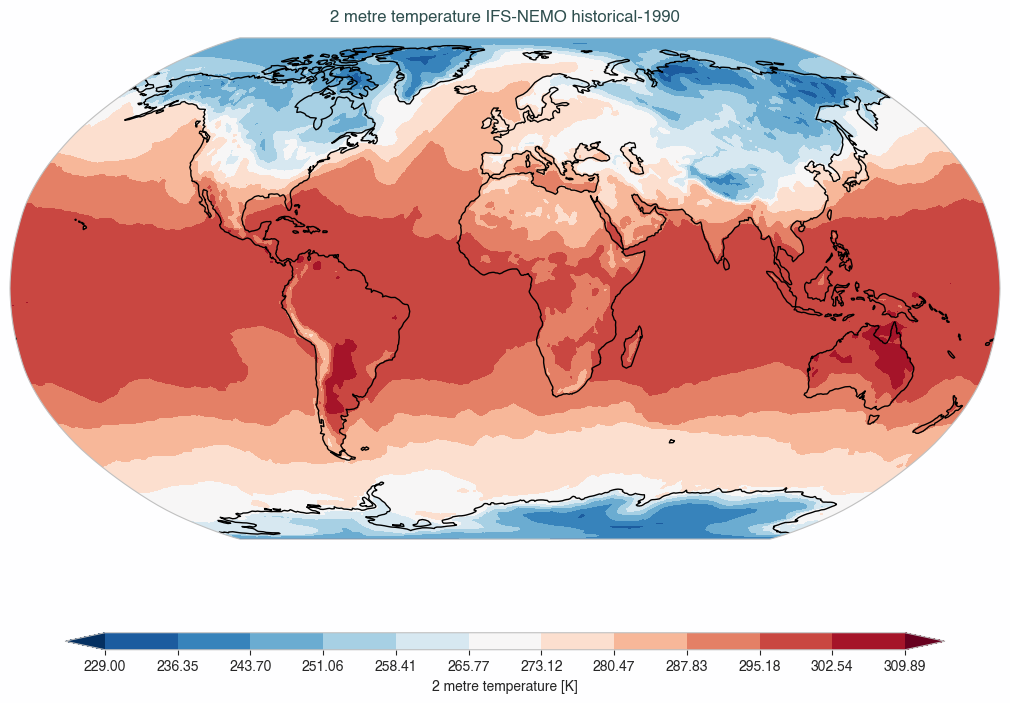
We can also interpolate the data to a 1°x1° grid and plot a timestep of it, all with AQUA tools.
data_2t_r = reader.regrid(data['2t']) # This is an xarray.DataArray
data_2t_r.isel(time=0).aqua.plot_single_map()
We used the regrid method to interpolate the data to a 1°x1° grid, with preprocessing of the weights already done
while initializating the Reader.
We then used the plot_single_map() function to plot the first timestep of the data.
This function has been used as accessor but can also be called as a standalone function.
See Accessors for more information.
Note
The regridding requires the download of auxiliary files containing the grids. Please refer to Access to aqua-dvc data for developers for more information on how to manage these files.
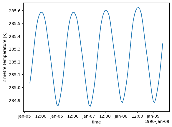
We can now calculate the mean global temperature time series on the original grid. We will use the original data, without regridding them, to show area evaluation capabilities of AQUA.
global_mean = reader.fldmean(data['2t'].isel(time=slice(100,200)))
global_mean.plot()
Note
Also for area evaluations, AQUA uses precomputed auxiliary files containing the area cells values. Please refer to Access to aqua-dvc data for developers for more information on how to manage these files.
We obtain as image:
For more detailed examples and tutorials, refer to the Examples and Tutorials section of this documentation or explore the Jupyter notebooks provided with AQUA.