Radiation Budget Diagnostic
Description
The Radiation is designed to evaluate radiative budget imbalances at the top of atmosphere (TOA) and at the surface (SFC).
Currently, the Radiation class includes only the function for generating boxplots, while time series and bias maps are produced by invoking other diagnostics in aqua-analysis using pecific configuration files.
The class can be extended in the future to incorporate additional radiation-specific features.
Structure
radiation.py: contains the Radiation classcli_radiation.py: the command line interface (CLI) script to run the diagnostic (boxplots only)
Input variables
Radiative fluxes are usually analyzed by this diagnostic (even though a boxplot can be done for any variable).:
tnlwrf: top net long-wave radiation flux (total thermal radiation) ;tnswrf: top net short-wave radiation flux (total solar radiation);tnr: top net radiation (difference between the two above);
The data we retrieve from the LRA through the provided functions have monthly timesteps and a 1x1 deg resolution. A higher resolution is not necessary for this diagnostic.
Basic usage
The basic usage of this diagnostic is explained with a working example in the notebook provided in the notebooks/diagnostics/radiation directory.
The basic structure of the analysis is the following:
from aqua import Reader
from aqua.diagnostics import  Radiation

#define and retrieve the data to use for the analysis
reader_ifs_nemo = Reader(model = 'IFS-NEMO', exp = 'historical-1990', source = 'lra-r100-monthly')
data_ifs_nemo = reader_ifs_nemo.retrieve()

reader_era5 = Reader(model="ERA5", exp="era5", source="monthly")
data_era5 = reader_era5.retrieve()

datasets = [data_ifs_nemo, data_era5, data_ceres]
model_names = ['IFS-NEMO', 'ERA5', 'CERES']
variables = ['-tnlwrf', 'tnswrf']

radiation = Radiation()
result = radiation.boxplot(datasets=datasets, model_names=model_names, variables=variables)
Note
A catalogs argument can be passed to the class to define the catalogs to use for the analysis.
If not provided, the Reader will identify the catalogs to use based on the models, experiments and sources provided.
CLI usage
The diagnostic can be run from the command line interface (CLI) by running the following command:
cd $AQUA/src/aqua_diagnostics/radiation
python radiation.py --config_file <path_to_config_file>
Additionally the CLI can be run with the following optional arguments:
--config,-c: Path to the configuration file.--nworkers,-n: Number of workers to use for parallel processing.--loglevel,-l: Logging level. Default isWARNING.--catalog: Catalog to use for the analysis. It can be defined in the config file.--model: Model to analyse. It can be defined in the config file.--exp: Experiment to analyse. It can be defined in the config file.--source: Source to analyse. It can be defined in the config file.--outputdir: Output directory for the plots.
Config file structure
The configuration file config_radiation-boxplots is a YAML file that contains the following information:
models: a list of models to analyse (defined by the catalog, model, exp, source arguments)
models:
  - catalog: climatedt-phase1
     model: IFS-NEMO
     exp: historical-1990
     source: lra-r100-monthly
  - catalog: obs
     model: ERA5
     exp: era5
     source: monthly
  - catalog: obs
     model: CERES
     exp: ebaf-toa41
     source: monthly
output: a block describing the details of the output. Is contains:outputdir: the output directory for the plots.rebuild: a boolean that enables the rebuilding of the plots.filename_keys: a list of keys for constructing the output filenames.save_netcdf: a boolean that enables the saving of the plots in NetCDF format.save_pdf: a boolean that enables the saving of the plots in pdf format.save_png: a boolean that enables the saving of the plots in png format.dpi: the resolution of the plots.
diagnostic_attributes: a block with the following information:variables: the list of variables to analyse.variable_names: the list of variable names to use in the plots.
Output
The diagnostic generates plots saved in PDF and png format as well as NetCDF files.
Observation
The diagnostic uses ERA5 and CERES as a default reference dataset for the radiation budget analysis. Custom reference datasets can be used.
References
Example plots
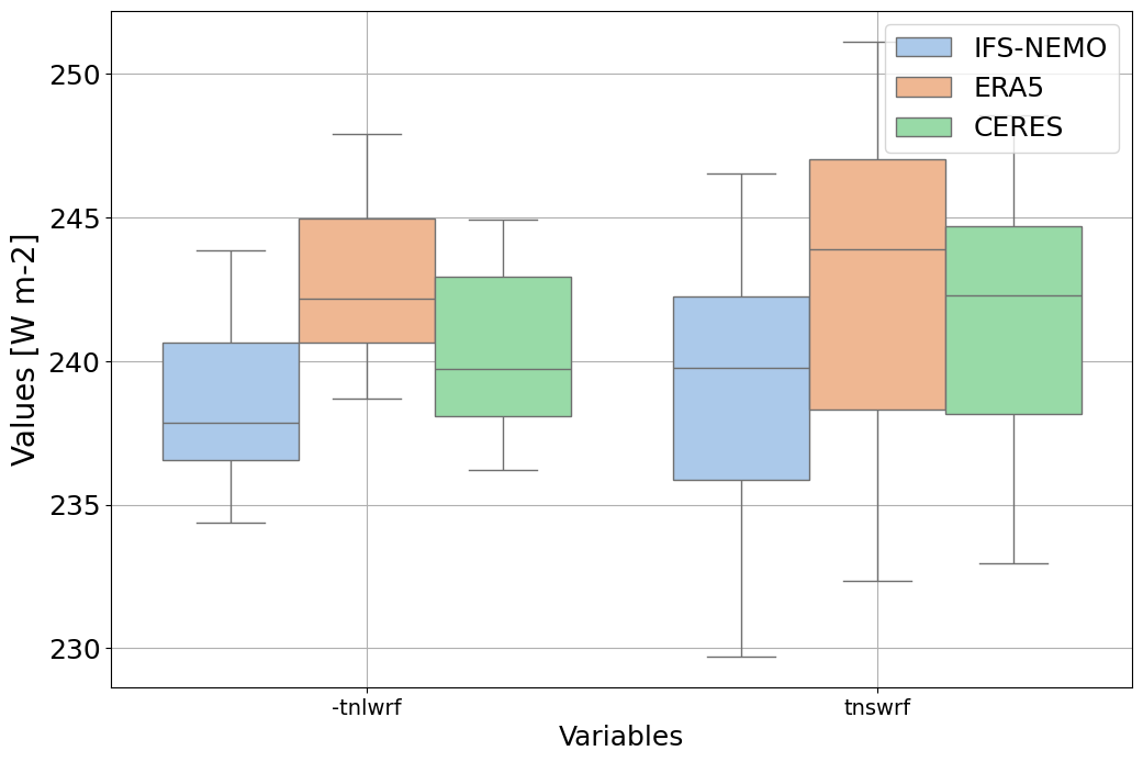
Box plot to show the globally averaged incoming and outgoing TOA radiation of IFS-NEMO historical-1990 with respect to ERA5 and CERES climatologies
Available demo notebooks
Notebooks are stored in diagnostics/global_biases/notebooks:
Detailed API
This section provides a detailed reference for the Application Programming Interface (API) of the Radiation diagnostic, produced from the diagnostic function docstrings.
- class aqua.diagnostics.radiation.Radiation
Bases:
object- boxplot(datasets=None, model_names=None, variables=None, variable_names=None, loglevel='WARNING')
Generate a boxplot showing the uncertainty of a global variable for different models.
- Parameters:
datasets (list of xarray.Dataset) – A list of xarray Datasets to be plotted.
model_names (list of str) – Names for the plotting, corresponding to the datasets.
variables (list of str) – List of variables to be plotted.
variable_names (list of str) – List of alternative names for the variables.
loglevel (str) – Logging level.
- Returns:
Matplotlib figure, axis objects, Pandas DataFrame of the processed boxplot data, and xarray Dataset of the boxplot data.
- Return type:
tuple