Global Biases Diagnostic

Description

The GlobalBiases diagnostic is a set of tools for the analysis and visualization of 2D spatial biases in climate model outputs. It supports comparative analysis between a target dataset (typically a climate model) and a reference dataset, commonly an observational or reanalysis product such as ERA5. Alternatively, it can be used to compare outputs from two different model simulations, for example to assess differences between historical and scenario experiments.

GlobalBiases provides tools to plot:

• Climatology maps

• Bias maps

• Seasonal bias maps

• Vertical profiles to assess biases across pressure levels

The diagnostic is designed with a class that analyzes a single model and generates the NetCDF files, and another class that produces the plots.

Classes

There is one class for the analysis and one for the plotting:

• GlobalBiases: the main class for the analysis of global biases. It retrieves the data and prepares it for plotting (e.g., regridding, pressure level selection, unit conversion). It also handles the computation of mean climatologies, including seasonal climatologies if requested. Climatologies are saved as class attributes and as NetCDF files.

• PlotGlobalBiases: this class provides methods for plotting the global biases, seasonal biases, and vertical profiles. It generates the plots based on the data prepared by the GlobalBiases class.

File structure

• The diagnostic is located in the src/aqua_diagnostics/global_biases directory, which contains both the source code and the command line interface (CLI) script.

• The configuration files are located in the config/diagnostics/global_biases directory and contain the default configuration for the diagnostic.

• Notebooks are available in the notebooks/diagnostics/global_biases directory and contain examples of how to use the diagnostic.

Input variables and datasets

By default, the diagnostic compares against the ERA5 dataset, but it can be configured to use any other dataset as a reference. A list of the variables that are compared automatically when running the full diagnostic is provided in the configuration files available in the config/diagnostics/global_biases directory.

Some of the variables that are typically used in this diagnostic are:

• 2m temperature (2t)

• Total Precipitation (tprate)

• Zonal and meridional wind (u, v)

• Specific humidity (q)

The diagnostic is designed to work with data from the Low Resolution Archive (LRA), generated by the Data reduction OPerator (DROP) of the AQUA project, which provides monthly data at a 1x1 degree resolution. A higher resolution is not necessary for this diagnostic.

Basic usage

The basic usage of this diagnostic is explained with a working example in the notebook provided in the notebooks/diagnostics/global_biases directory. The basic structure of the analysis is the following:

from aqua.diagnostics import GlobalBiases, PlotGlobalBiases

biases_ifs_nemo = GlobalBiases(model='IFS-NEMO', exp='historical-1990', source='lra-r100-monthly', loglevel="DEBUG")
biases_era5 = GlobalBiases(model='ERA5', exp='era5', source='monthly', startdate="1990-01-01", enddate="1999-12-31", loglevel="DEBUG")

biases_ifs_nemo.retrieve(var='q')
biases_ifs_nemo.compute_climatology(seasonal=True)

biases_era5.retrieve(var='q')
biases_era5.compute_climatology(seasonal=True)

pg = PlotGlobalBiases(loglevel='DEBUG')
pg.plot_bias(data=biases_ifs_nemo.climatology, data_ref=biases_era5.climatology, var='q', plev=18000)

Note

The user can also define the start and end date of the analysis and the reference dataset. If not specified otherwise, plots will be saved in PNG and PDF format in the current working directory.

CLI usage

The diagnostic can be run from the command line interface (CLI) by running the following command:

cd $AQUA/src/aqua_diagnostics/global_biases
python cli_global_biases.py --config_file <path_to_config_file>

Additionally, the CLI can be run with the following optional arguments:

• --config, -c: Path to the configuration file.

• --nworkers, -n: Number of workers to use for parallel processing.

• --cluster: Cluster to use for parallel processing. By default a local cluster is used.

• --loglevel, -l: Logging level. Default is WARNING.

• --catalog: Catalog to use for the analysis. Can be defined in the config file.

• --model: Model to analyse. Can be defined in the config file.

• --exp: Experiment to analyse. Can be defined in the config file.

• --source: Source to analyse. Can be defined in the config file.

• --outputdir: Output directory for the plots.

Config file structure

The configuration file is a YAML file that contains the details on the dataset to analyse or use as reference, the output directory and the diagnostic settings. Most of the settings are common to all the diagnostics (see Diagnostics configuration files). Here we describe only the specific settings for the global biases diagnostic.

• globalbiases: a block (nested in the diagnostics block) containing options for the Global Biases diagnostic. Variable-specific parameters override the defaults.

  • run: enable/disable the diagnostic.

  • diagnostic_name: name of the diagnostic. globalbiases by default, but can be changed when the boxplots CLI is invoked within another recipe diagnostic, as is currently done for Radiation.

  • variables: list of variables to analyse.

  • formulae: list of formulae to compute new variables from existing ones (e.g., tnlwrf+tnswrf).

  • plev: pressure levels to analyse for 3D variables.

  • seasons: enable seasonal analysis.

  • seasons_stat: statistic to use for seasonal climatology (e.g., “mean”).

  • vertical: enable vertical profiles.

  • startdate_data / enddate_data: time range for the dataset.

  • startdate_ref / enddate_ref: time range for the reference dataset.

globalbiases:
    run: true
    diagnostic_name: 'globalbiases'
    variables: ['tprate', '2t', 'msl', 'tnlwrf', 't', 'u', 'v', 'q', 'tos']
    formulae: ['tnlwrf+tnswrf']
    params:
        default:
            plev: [85000, 20000]
            seasons: true
            seasons_stat: 'mean'
            vertical: true
            startdate_data: null
            enddate_data: null
            startdate_ref: "1990-01-01"
            enddate_ref: "2020-12-31"
        tnlwrf+tnswrf:
            short_name: "tnr"
            long_name: "Top net radiation"

• plot_params: defines colorbar palette and limits and projection parameters for each variable. The default parameters are used if not specified for a specific variable. Refer to ‘src/aqua/util/projections.py’ for available projections.

plot_params:
    default:
        projection: 'robinson'
        projection_params: {}
    2t:
        cmap: 'RdBu_r'
        vmin: -15
        vmax: 15
    msl:
        vmin: -1000
        vmax: 1000
    u:
        vmin_v: -50
        vmax_v: 50

Output

The diagnostic produces four types of plots:

• Global climatology maps

• Global bias maps (model vs reference)

• Seasonal bias maps

• Vertical bias profiles (for 3D variables)

Plots are saved in both PDF and PNG format.

Observations

The default reference dataset is ERA5, but custom references can be configured.

Example Plots

All plots can be reproduced using the notebooks in the notebooks directory on LUMI HPC.

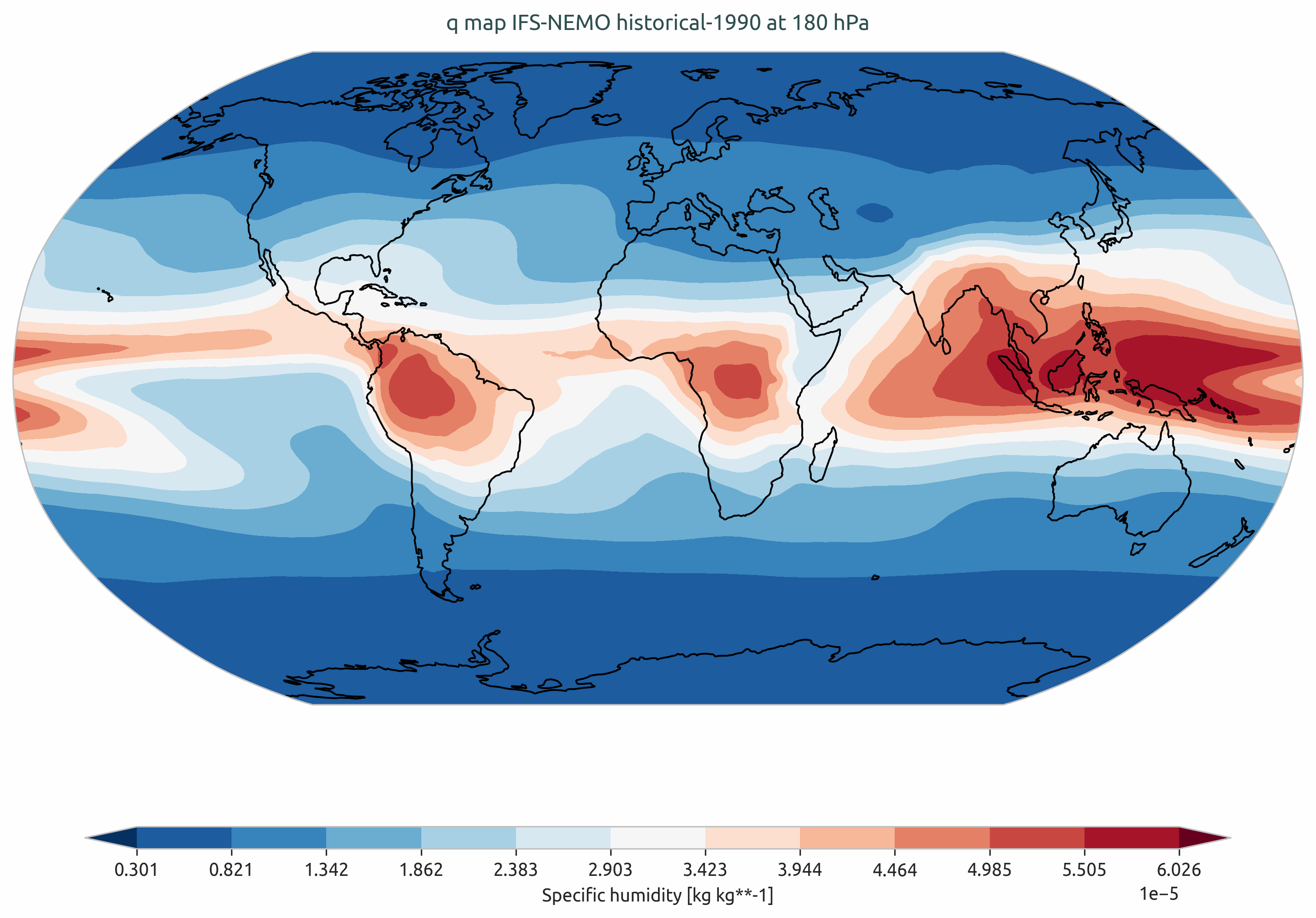
Climatology of q from IFS-NEMO historical-1990.

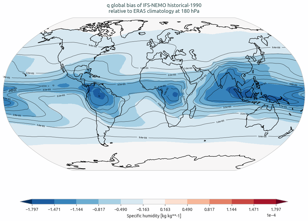
Global bias of q from IFS-NEMO historical-1990 with respect to ERA5 climatology.

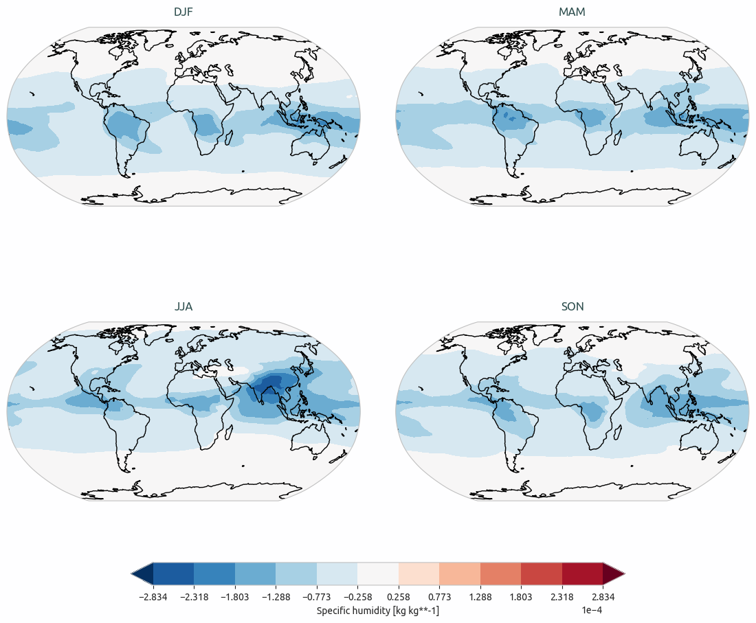
Seasonal bias of q from IFS-NEMO historical-1990 with respect to ERA5 climatology.

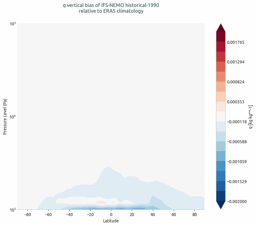
Vertical bias of q from IFS-NEMO historical-1990 with respect to ERA5 climatology.

Available demo notebooks

Notebooks are stored in the notebooks/diagnostics/global_biases directory and contain usage examples.

• global_biases.ipynb

Authors and contributors

This diagnostic is maintained by Silvia Caprioli (@silviacaprioli, silvia.caprioli@polito.it). Contributions are welcome — please open an issue or a pull request. For questions or suggestions, contact the AQUA team or the maintainers.

Detailed API

This section provides a detailed reference for the Application Programming Interface (API) of the global_biases diagnostic, generated from the function docstrings.

class aqua.diagnostics.global_biases.GlobalBiases(catalog=None, model=None, exp=None, source=None, regrid=None, startdate=None, enddate=None, var=None, plev=None, diagnostic='globalbiases', save_netcdf=True, outputdir='./', loglevel='WARNING')

Bases: Diagnostic

Diagnostic class for computing global and seasonal climatologies of a given variable.

This class handles data retrieval, pressure level selection, unit conversion, and computation of mean climatologies (total or seasonal).

Inherits from Diagnostic.

Parameters:

• catalog (str) – The catalog to be used. If None, inferred from Reader.

• model (str) – Model to be used.

• exp (str) – Experiment name.

• source (str) – Source name.

• regrid (str) – Target grid for regridding. If None, no regridding.

• startdate (str) – Start date for data selection.

• enddate (str) – End date for data selection.

• var (str) – Variable name to analyze.

• plev (float) – Pressure level to select (if applicable).

• diagnostic (str) – Name of the diagnostic.

• save_netcdf (bool) – If True, saves output climatologies.

• outputdir (str) – Output directory for NetCDF files.

• loglevel (str) – Log level. Default is ‘WARNING’.

Initialize the diagnostic class. This is a general purpose class that can be used by the diagnostic classes to retrieve data from a single model and to save the data to a netcdf file. It is not a working diagnostic class by itself.

Parameters:

• model (str) – The model to be used.

• exp (str) – The experiment to be used.

• source (str) – The source to be used.

• catalog (str) – The catalog to be used. If None, the catalog will be determined by the Reader.

• regrid (str | None) – The target grid to be used for regridding. If None, no regridding will be done.

• startdate (str | None) – The start date of the data to be retrieved. If None, all available data will be retrieved.

• enddate (str | None) – The end date of the data to be retrieved. If None, all available data will be retrieved.

• loglevel (str) – The log level to be used. Default is ‘WARNING’.

compute_climatology(data: Dataset = None, var: str = None, plev: float = None, save_netcdf: bool = None, seasonal: bool = False, seasons_stat: str = 'mean', create_catalog_entry: bool = False) → None

Compute total and optionally seasonal climatology for a variable.

Parameters:

• data (xarray.Dataset, optional) – Input dataset. If None, uses self.data.

• var (str, optional) – Variable name. If None, uses self.var.

• plev (float, optional) – Pressure level (currently unused).

• save_netcdf (bool, optional) – If True, save output to NetCDF.

• seasonal (bool) – If True, compute seasonal climatology (DJF, MAM, JJA, SON).

• seasons_stat (str) – Aggregation statistic: ‘mean’, ‘std’, ‘max’, ‘min’.

• create_catalog_entry (bool) – If True, create a catalog entry for the data. Default is False.

Raises:

ValueError – If seasons_stat is invalid.

retrieve(var: str = None, formula: bool = False, long_name: str = None, short_name: str = None, plev: float = None, units: str = None, reader_kwargs: dict = {}) → None

Retrieve and preprocess dataset, selecting pressure level and/or converting units if needed.

Parameters:

• var (str, optional) – Variable to retrieve. If None, uses self.var.

• formula (bool) – If True, the variable is a formula.

• long_name (str) – The long name of the variable, if different from the variable name.

• short_name (str) – The short name of the variable, if different from the variable name.

• plev (float, optional) – Pressure level to extract.

• units (str) – The units of the variable, if different from the original units.

• reader_kwargs (dict, optional) – Additional keyword arguments for the Reader.

Raises:

• NoDataError – If variable not found in dataset.

• KeyError – If the variable is missing from the data.

savenetcdf(data: Dataset, diagnostic_product: str, rebuild: bool = True, create_catalog_entry: bool = False, extra_keys=None, dict_catalog_entry: dict = {'jinjalist': ['realization'], 'wildcardlist': ['var']})

data (xr.Dataset): Input dataset. diagnostic_product (str): The product name to be used in the filename (e.g., ‘annual_climatology’). rebuild (bool): If True, rebuild the data from the original files. create_catalog_entry (bool): If True, create a catalog entry for the data. Default is False. extra_keys (dict): Extra keys for filename generation. dict_catalog_entry (dict): A dictionary with catalog entry information.

Default is {‘jinjalist’: [‘freq’, ‘region’, ‘realization’], ‘wildcardlist’: [‘var’]}.

class aqua.diagnostics.global_biases.PlotGlobalBiases(diagnostic='globalbiases', save_pdf=True, save_png=True, dpi=300, outputdir='./', cmap='RdBu_r', loglevel='WARNING')

Bases: object

Initialize the PlotGlobalBiases class.

Parameters:

• diagnostic (str) – Name of the diagnostic.

• save_pdf (bool) – Whether to save the figure as PDF.

• save_png (bool) – Whether to save the figure as PNG.

• dpi (int) – Resolution of saved figures.

• outputdir (str) – Output directory for saved plots.

• cmap (str) – Colormap to use for the plots.

• loglevel (str) – Logging level.

plot_bias(data, data_ref, var, plev=None, proj='robinson', proj_params={}, vmin=None, vmax=None, cbar_label=None)

Plots the bias map between two datasets.

Parameters:

• data (xarray.Dataset) – Primary dataset.

• data_ref (xarray.Dataset) – Reference dataset.

• var (str) – Variable name.

• plev (float, optional) – Pressure level.

• proj (str, optional) – Desired projection for the map.

• proj_params (dict, optional) – Additional arguments for the projection.

• vmin (float, optional) – Minimum colorbar value.

• vmax (float, optional) – Maximum colorbar value.

• cbar_label (str, optional) – Label for the colorbar.

plot_climatology(data, var, plev=None, proj='robinson', proj_params={}, vmin=None, vmax=None, cbar_label=None)

Plots the climatology map for a given variable and time range.

Parameters:

• data (xarray.Dataset) – Climatology dataset to plot.

• var (str) – Variable name.

• plev (float, optional) – Pressure level to plot (if applicable).

• proj (string, optional) – Desired projection for the map.

• proj_params (dict, optional) – Additional arguments for the projection (e.g., {‘central_longitude’: 0}).

• vmin (float, optional) – Minimum color scale value.

• vmax (float, optional) – Maximum color scale value.

• cbar_label (str, optional) – Label for the colorbar.

Returns:

Matplotlib figure and axis objects.

Return type:

tuple

plot_seasonal_bias(data, data_ref, var, plev=None, proj='robinson', proj_params={}, vmin=None, vmax=None, cbar_label=None)

Plots seasonal biases for each season (DJF, MAM, JJA, SON).

Parameters:

• data (xarray.Dataset) – Primary dataset.

• data_ref (xarray.Dataset) – Reference dataset.

• var (str) – Variable name.

• plev (float, optional) – Pressure level.

• proj (str, optional) – Desired projection for the map.

• proj_params (dict, optional) – Additional arguments for the projection.

• vmin (float, optional) – Minimum colorbar value.

• vmax (float, optional) – Maximum colorbar value.

• cbar_label (str, optional) – Label for the colorbar.

Returns:

The resulting figure.

Return type:

matplotlib.figure.Figure

plot_vertical_bias(data, data_ref, var, plev_min=None, plev_max=None, vmin=None, vmax=None, vmin_contour=None, vmax_contour=None, nlevels=18)

Calculates and plots the vertical bias between two datasets.

Parameters:

• data (xarray.Dataset) – Dataset to analyze.

• data_ref (xarray.Dataset) – Reference dataset for comparison.

• var (str) – Variable name to analyze.

• plev_min (float, optional) – Minimum pressure level.

• plev_max (float, optional) – Maximum pressure level.

• vmin (float, optional) – Minimum colorbar value.

• vmax (float, optional) – Maximum colorbar value.

• vmin_contour (float, optional) – Minimum contour value.

• vmax_contour (float, optional) – Maximum contour value.

• nlevels (int, optional) – Number of contour levels for the plot.