Ensemble Statistics

Description

The Ensemble module is a tool to perform uncertainty quantification and visualising the ensemble statistics namely, mean and standard deviation. It is also possible to calculate the weighted mean and standard deviation in case of multi-model ensemble. This module contains three main classes namely, EnsembleTimeseries, EnsembleLatLon and EnsembleZonal. Additionally, this module also contains three supporting plotting classes namely, PlotEnsembleTimeseries, PlotEnsembleLatLon and PlotEnsembleZonal.

The EnsembleTimeseries class takes 1D xarray.Dataset timeseries as input and performs following functionalities: - Computes ensemble mean and standard deviation (Point-wise along time axis) for monthly and annual timeseries.

The PlotEnsembleTimeseries class takes 1D xarray.Dataset timeseries as input and performs the following functionalities: - Plots the ensemble-mean and 2x ensemble-std ± ensemble-mean along the given timeseries. - Note that the standard deviation is Point-wise along time axis. - A reference timeseries can also be plotted.

The EnsembleLatLon class takes 2D LatLon xarray.Dataset as input and performs the following functionalities: - Compute ensemble mean and standard deviation for 2D Maps.

The PlotEnsembleLatLon class takes 2D LatLon xarray.Dataset as input and performs the following functionalities: - Plots the ensemble mean and standard deviation separately on two different maps.

The EnsembleZonal class take zonal-averages Lev-Lon xarray.Dataset as input and performs the following functionalities: - Computes ensemble mean and standard deviation of the given input.

The PlotEnsembleZonal class take zonal-averages Lev-Lon xarray.Dataset as input and performs the following functionalities: - Plots the ensemble mean and standard deviation of the computed statistics.

Structure

ensembleTimeseries.py: contains the EnsembleTimeseries class.
plot_ensemble_timeseries.py: contains the PlotEnsembleTimeseries class.
ensembleLatLon.py: contains the EnsembleLatLon class.
plot_ensemble_latlon.py: contains the PlotEnsembleLatLon.py class.
ensembleZonal.py: contains the EnsembleZonal class.
plot_ensemble_zonal.py: contains the PlotEnsembleLatLon.py class.
cli_multi_model_timeseries_ensemble: the command line interfance (CLI) script to run the ensemble-timeseries 1D diagnostic (mulit-model).
cli_single_model_timeseries_ensemble: the command line interfance (CLI) script to run the ensemble-timeseries 1D diagnostic (single-model-ensemble).
cli_global_2D_ensemble.py: the command line interfance (CLI) script to run the ensemble-2D-maps in Lat-Lon diagnostic.
cli_zonal_ensemble.py: the command line interfance (CLI) script to run the ensemble-zonal Lev-Lon diagnostic.
util.py: contains the reader_retrieve_and_merge, merge_from_data_files and compute_statistics functions.
base.py: contains the base class which contains functions for saving the output as png, pdf and netcdf.
config/diagnostics/ensemble/config_global_2D_ensemble.yaml: config file for cli_global_2D_ensemble.py.
config/diagnostics/ensemble/config_multi_model_timeseries_ensemble.yaml: config file for ensembleTimeseries.py.
config/diagnostics/ensemble/config_single_model_timeseries_ensemble.yaml: config file for ensembleTimeseries.py.
config/diagnostics/ensemble/config_zonalmean_ensemble.yaml: config file for ensembleZonal.py.

Input variables

In order to use the Ensemble module, a pre-processing step is required. To load and to merge the input data via Reader class use aqua.diagnostics.ensemble.util.reader_retrieve_and_merge. Additional functionality of this module is to load and merge using the list of paths of data via merge_from_data_files. In this step one has to merge all the given 1D timeseries, 2D Lat-Lon Map and Zonal-averages Lev-Lon for EnsembleTimeseries, EnsembleLatLon and EnsembleZonal along a pesudo-dimension, respectively. The default dimension is simply named as ensemble and can be changed. One can load the data directly as xarray.Dataset or can use the aqua Reader class. For example loading and merging a 2D maps ensemble into an xarray.Dataset:

import glob
from  aqua.diagnostics import merge_from_data_files

file_list = glob.glob('/work/ab0995/a270260/pre_computed_aqua_analysis/*/historical-1990/atmglobalmean/netcdf/atmglobalmean.statistics_maps.2t.*_historical-1990.nc')
file_list.sort()
ens_dataset = merge_from_data_files(
    variable='2t',
    model_names= ['IFS-FESOM', 'IFS-NEMO'],
    data_path_list=file_list,
    log_level = "WARNING",
    ens_dim="ensemble",
)

A second method:

from  aqua.diagnostics import reader_retrieve_and_merge

ens_dataset = reader_retrieve_and_merge(
    variable='2t',
    catalog_list=['nextgems4', 'climatedt-phase1'],
    models_catalog_list=['IFS-FESOM', 'IFS-NEMO'],
    exps_catalog_list=['historical-1990', 'historical-1990'],
    sources_catalog_list=['aqua-atmglobalmean', 'aqua-atmglobalmean'],
    log_level="WARNING",
    ens_dim="ensemble",
)

Ensemble computation

The ensemble statistics is performed on merged 1D timesereies by EnsembleTimeseries, 2D map by EnsembleLatLon, and zonal Lev-Lon by EnsembleZonal classes. Note that in the current version we provide point-wise ensemble mean and standard-deviation.

from aqua.diagnostics import EnsembleTimeseries

# Check if we need monthly and annual time variables
ts = EnsembleTimeseries(
    var=variable,
    model_list=['IFS-FESOM', 'IFS-NEMO'],
    monthly_data=mon_model_dataset,
    annual_data=ann_model_dataset,
    outputdir='./',
    loglevel='WARNING',
)

# Compute statistics and save the results as netcdf
ts.run()

Ensemble Plotting

The default values for the plotting fuction has been already set as default values. These values can also be by simply defining a python dictionary e.g., in the case of the EnsembleTimeseries, plot_options = {'plot_ensemble_members': True, 'ensemble_label': 'Multi-model', 'plot_title': 'Ensemble statistics for 2-meter temperature [K]', 'ref_label': 'ERA5', 'figure_size': [12,6]}.

For EnsembleLatLon, plot_options = {'figure_size': [15,14], 'cbar_label': '2-meter temperature in K','mean_plot_title': 'Map of 2t for Ensemble Multi-Model mean', 'std_plot_title': 'Map of 2t for Ensemble Multi-Model standard deviation'}.

For EnsembleZonal, plot_options = {'figure_size': [12,8], 'plot_label': True, 'plot_std': True, 'unit': None, 'mean_plot_title': 'Mean of Ensemble of Zonal average', 'std_plot_title': 'Standard deviation of Ensemble of Zonal average', 'cbar_label': 'temperature in K', 'dpi': 300}.

from aqua.diagnostics import PlotEnsembleTimeseries
# PlotEnsembleTimeseries class
plot_class_arguments = {
    "model_list": ['IFS-FESOM', 'IFS-NEMO'],
    "ref_model": 'ERA5',
}

plot_arguments = {
    "var": variable,
    "save_pdf": True,
    "save_png": True,
    "plot_ensemble_members": True,
    "monthly_data": ts.monthly_data,
    "monthly_data_mean": ts.monthly_data_mean,
    "monthly_data_std": ts.monthly_data_std,
    "annual_data": ts.annual_data,
    "annual_data_mean": ts.annual_data_mean,
    "annual_data_std": ts.annual_data_std,
    "ref_monthly_data": mon_ref_data,
    "ref_annual_data": ann_ref_data,}

ensemble_plot = ts_plot.plot(**plot_arguments)


ts_plot = PlotEnsembleTimeseries(
    **plot_class_arguments,
    loglevel='WARNING',
)

Ensemble module provides output plots as PDF and PNG.

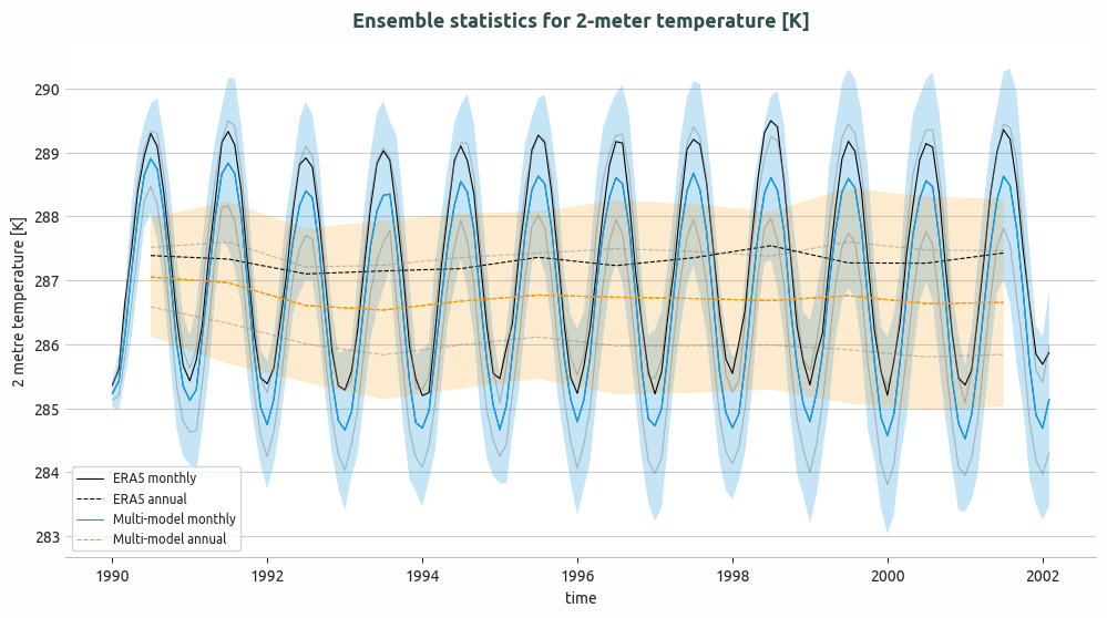
../_images/ensemble_time_series_timeseries_2t.png — Ensemble of multi-model global monthly and annual timeseries and compared with ERA5 global monthly and annual average. Models considered as IFS-NEMO and IFS-FESOM.

Basic usage

The basic usage of this diagnostics is explained with working examples in the notebooks provided in notebooks/diagnostics/ensemble directory. Additionally, a detailed command line interface is also avaiable in src/aqua_diagnostics/ensemble directory.

Notebooks are stored in notebooks/ensemble:

ensemble_timeseries.ipynb <https://github.com/DestinE-Climate-DT/AQUA/blob/main/notebooks/diagnostics/ensemble/ensemble_timeseries.ipynb> _
ensemble_global_2D.ipynb <https://github.com/DestinE-Climate-DT/AQUA/blob/main/notebooks/diagnostics/ensemble/ensemble_global_2D.ipynb> _
ensemble_zonalaverage.ipynb <https://github.com/DestinE-Climate-DT/AQUA/blob/main/notebooks/diagnostics/ensemble/ensemble_zonalaverage.ipynb> _

Example Plots

Other example of ensemble module provides output plots as PDF and PNG.

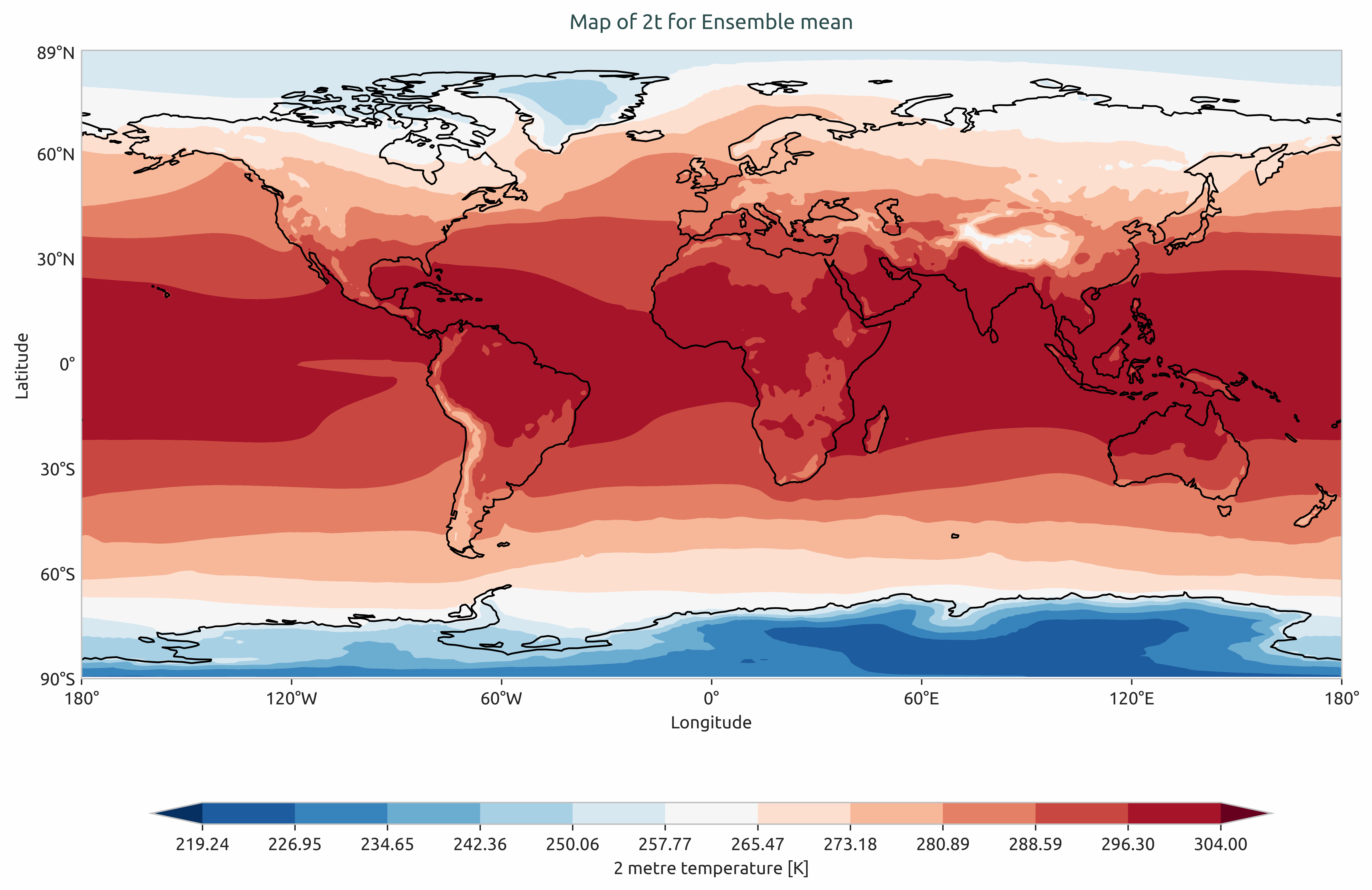
../_images/2t_LatLon_mean.png — Ensemble mean of multi-model of global mean of 2-meter temperature. Models considered as IFS-NEMO and IFS-FESOM.

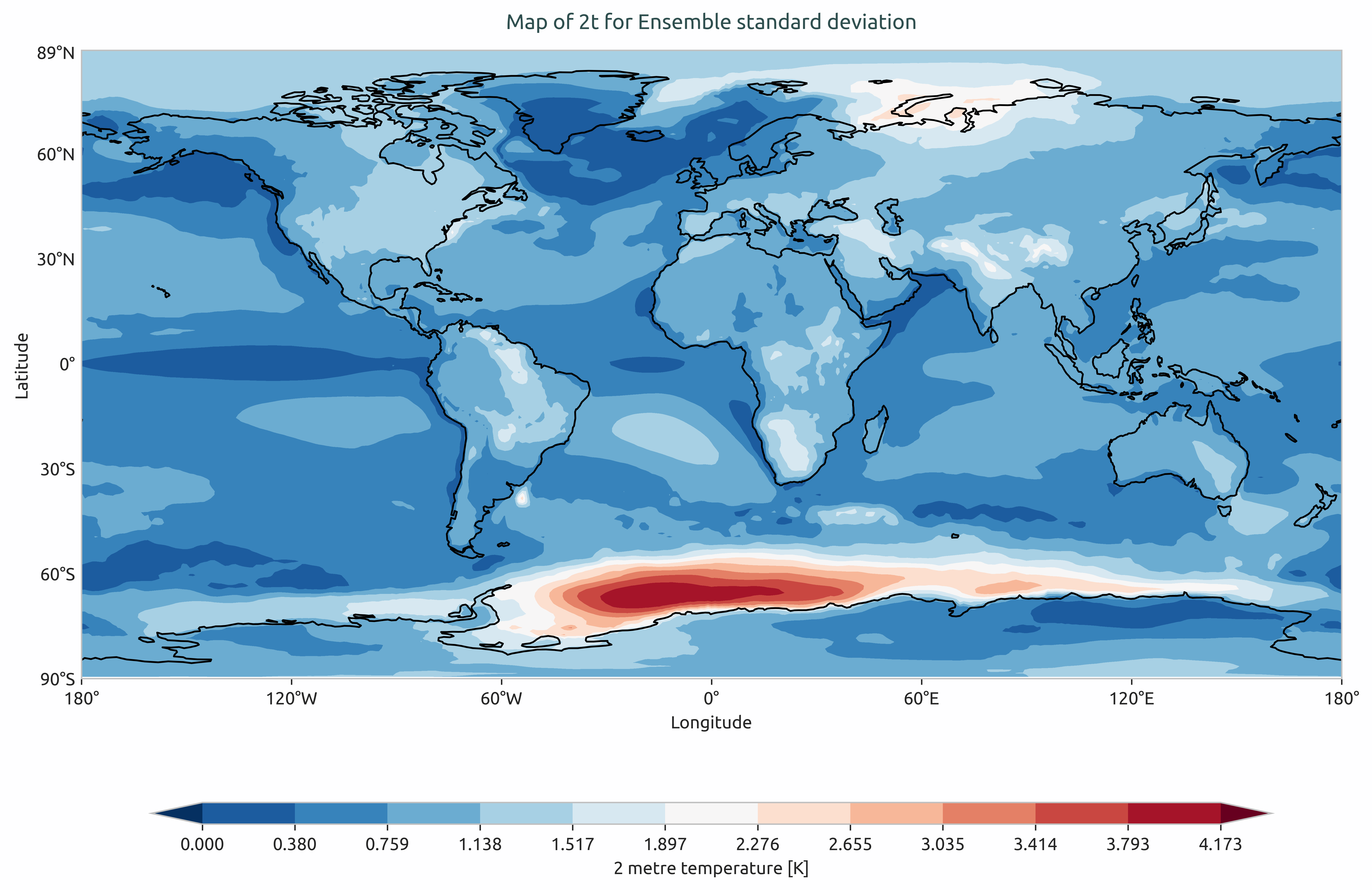
../_images/2t_LatLon_STD.png — Ensemble standard devation of multi-model of the global mean of 2-meter temperature. Models considered as IFS-NEMO and IFS-FESOM.

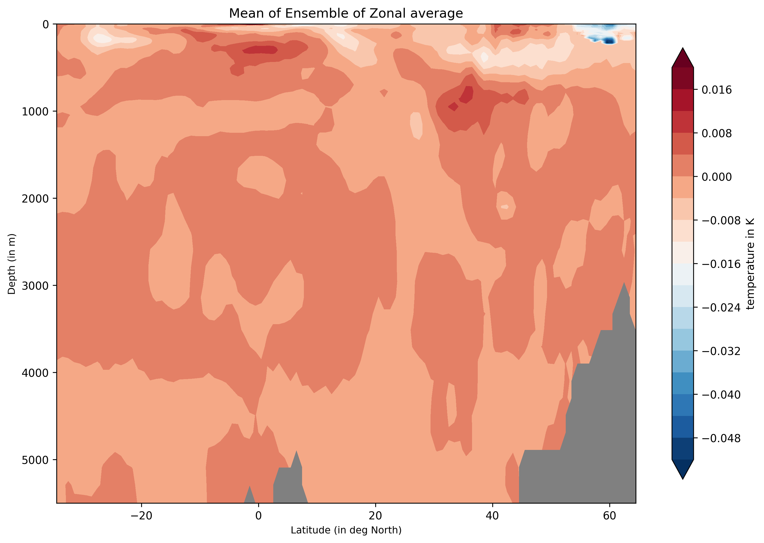
../_images/avg_so_LevLon_mean.png — Ensemble-Zonal mean for average Time-mean sea water practical salinity for IFS-NEMO historical-1990.

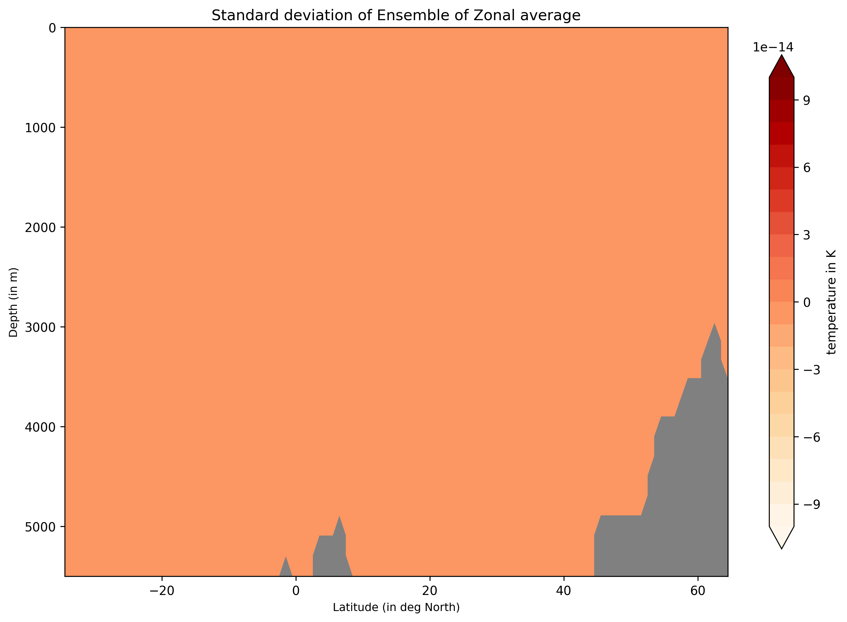
../_images/avg_so_LevLon_STD.png — Ensemble-Zonal standard deviation for average Time-mean sea water practical salinity for IFS-NEMO historical-1990.

Detailed API

This section provides a detailed reference for the Application Programming Interface (API) of the ensemble diagnostic, produced from the diagnostic function docstrings.

class aqua.diagnostics.ensemble.EnsembleLatLon(var=None, dataset=None, catalog_list=None, model_list=None, exp_list=None, source_list=None, ensemble_dimension_name='ensemble', description=None, outputdir='./', loglevel='WARNING')

Bases: BaseMixin

A class to compute ensemble mean and standard deviation of a 2D (lon-lat) Dataset. Make sure that the dataset has correct lon-lat dimensions.

Parameters:

var (str) – Variable name.
dataset – xarray Dataset composed of ensembles 2D lon-lat data, i.e., the individual Dataset (lon-lat) are concatenated along. a new dimension “ensemble”. This ensemble name can be changed.
catalog_list (str) – This variable defines the catalog list. The default is ‘None’. If None, the variable is assigned to ‘None_catalog’. In case of Multi-catalogs, the variable is assigned to ‘multi-catalog’.
model_list (str) – This variable defines the model list. The default is ‘None’. If None, the variable is assigned to ‘None_model’. In case of Multi-Model, the variable is assigned to ‘multi-model’.
exp_list (str) – This variable defines the exp list. The default is ‘None’. If None, the variable is assigned to ‘None_exp’. In case of Multi-Exp, the variable is assigned to ‘multi-exp’.
source_list (str) – This variable defines the source list. The default is ‘None’. If None, the variable is assigned to ‘None_source’. In case of Multi-Source, the variable is assigned to ‘multi-source’.
ensemble_dimension_name="ensemble" (str) – a default name given to the dimensions along with the individual Datasets were concatenated.
outputdir (str) – String input for output path.
description (str) – Description of the netcdf.
loglevel (str) – Log level. Default is “WARNING”.

run(): A function to compute the mean and standard devivation of the input dataset It is import to make sure that the dim along which the mean is compute is correct. The default dim=”ensemble”.

class aqua.diagnostics.ensemble.EnsembleTimeseries(var=None, hourly_data=None, daily_data=None, monthly_data=None, annual_data=None, catalog_list=None, model_list=None, exp_list=None, source_list=None, ensemble_dimension_name='ensemble', description=None, outputdir='./', loglevel='WARNING')

Bases: BaseMixin

This class computes mean and standard deviation of the timeseries ensemble.

NOTE: The STD is computed Point-wise along the mean.

Parameters:

var (str) – Variable name.
hourly_data – xarray Dataset of ensemble members of hourly timeseries. The ensemble memebers are concatenated along a new dimension “ensemble”.
daily_data – xarray Dataset of ensemble members of daily timeseries. The ensemble memebers are concatenated along a new dimension “ensemble”.
monthly_data – xarray Dataset of ensemble members of monthly timeseries. The ensemble memebers are concatenated along a new dimension “ensemble”.
annual_data – xarray Dataset of ensemble members of annual timeseries. The ensemble members are concatenated along the dimension “ensemble”
ensemble_dimension_name="ensemble" (str) – a default name given to the dimensions along with the individual Datasets were concatenated.
catalog_list (list) – list of catalog names.
model_list (list) – list of model names. This is mandotory.
exp_list (list) – list of experiment names.
source_list (list) – list of source list.
description (str) – Description of the netcdf.
outputdir (str) – String input for output path.
loglevel (str) – Log level. Default is “WARNING”.

run(): A function to compute the mean and standard devivation of the input dataset It is import to make sure that the dim along which the mean is compute is correct. The default dim=”ensemble”. TODO: Test DASK’s .compute() function here.

class aqua.diagnostics.ensemble.EnsembleZonal(var=None, dataset=None, catalog_list=None, model_list=None, exp_list=None, source_list=None, ensemble_dimension_name='ensemble', outputdir='./', loglevel='WARNING')

Bases: BaseMixin

A class to compute ensemble mean and standard deviation of the Zonal averages Make sure that the dataset has correct lev-lat dimensions.

Parameters:

var (str) – Variable name.
dataset – xarray Dataset composed of ensembles 2D Zonal data, i.e., the individual Dataset (lev-lat) are concatenated along. a new dimension “ensemble”. This ensemble name can be changed.
catalog_list (str) – This variable defines the catalog list. The default is ‘None’. If None, the variable is assigned to ‘None_catalog’. In case of Multi-catalogs, the variable is assigned to ‘multi-catalog’.
model_list (str) – This variable defines the model list. The default is ‘None’. If None, the variable is assigned to ‘None_model’. In case of Multi-Model, the variable is assigned to ‘multi-model’.
exp_list (str) – This variable defines the exp list. The default is ‘None’. If None, the variable is assigned to ‘None_exp’. In case of Multi-Exp, the variable is assigned to ‘multi-exp’.
source_list (str) – This variable defines the source list. The default is ‘None’. If None, the variable is assigned to ‘None_source’. In case of Multi-Source, the variable is assigned to ‘multi-source’.
ensemble_dimension_name="ensemble" (str) – a default name given to the dimensions along with the individual Datasets were concatenated.
outputdir (str) – String input for output path.
loglevel (str) – Log level. Default is “WARNING”.

run(): A function to compute the mean and standard devivation of the input dataset It is import to make sure that the dim along which the mean is compute is correct. The default dim=”ensemble”.

class aqua.diagnostics.ensemble.PlotEnsembleLatLon(diagnostic_product: str = 'EnsembleLatLon', catalog_list: list[str] = None, model_list: list[str] = None, exp_list: list[str] = None, source_list: list[str] = None, region: str = None, outputdir='./', loglevel: str = 'WARNING')

Bases: BaseMixin

Class to plot the ensmeble lat-lon

Class for plotting ensemble latitude-longitude (Lat-Lon) data.

This class inherits from BaseMixin and provides functionality to generate plots of ensemble datasets on a latitude-longitude grid. It supports multiple catalogs, models, experiments, and sources, and allows saving plots as PNG or PDF files. The class is intended for ensemble statistics visualization, such as mean and standard deviation maps.

Parameters:

diagnostic_product (str, optional) – Name of the diagnostic product. Defaults to “EnsembleLatLon”.
catalog_list (list[str], optional) – List of catalog names. If None, assigned to ‘None_catalog’.
model_list (list[str], optional) – List of model names. If None, assigned to ‘None_model’.
exp_list (list[str], optional) – List of experiment names. If None, assigned to ‘None_exp’.
source_list (list[str], optional) – List of data source names. If None, assigned to ‘None_source’.
region (str, optional) – Name of the region for plotting. Defaults to None.
outputdir (str, optional) – Directory to save output plots. Defaults to “./”.
loglevel (str, optional) – Logging level. Defaults to “WARNING”.

figure

The figure object for the plot.

Type:: matplotlib.figure.Figure or None

diagnostic_product

Name of the diagnostic product being visualized.

Type:: str

catalog_list

List of catalogs being processed.

Type:: list[str]

model_list

List of models being processed.

Type:: list[str]

exp_list

List of experiments being processed.

Type:: list[str]

source_list

List of sources being processed.

Type:: list[str]

region

Region name for plotting.

Type:: str

outputdir

Directory path for saving plots.

Type:: str

loglevel

Logging level for messages.

Type:: str

Notes

Designed to visualize ensemble mean and standard deviation on Lat-Lon grids.
Integrates with BaseMixin for consistent handling of catalogs, models, and experiments.
Uses self.save_figure for saving output plots in PNG and PDF formats.

plot(var: str = None, dataset_mean=None, dataset_std=None, long_name=None, description=None, dpi=300, title_mean=None, title_std=None, save_pdf=True, save_png=True, vmin_mean=None, vmax_mean=None, vmin_std=None, vmax_std=None, proj='robinson', proj_params={}, transform_first=False, cyclic_lon=True, contour=True, coastlines=True, cbar_label=None, units=None)

Plot ensemble mean and standard deviation on a latitude-longitude map.

Generates 2D maps of ensemble mean and standard deviation for a given variable using the specified projection and visualization options. The resulting figures can be saved as PNG and/or PDF files.

Parameters:

var (str) – Variable name to plot.
dataset_mean (xarray.DataArray or Dataset) – Ensemble mean dataset.
dataset_std (xarray.DataArray or Dataset) – Ensemble standard deviation dataset.
long_name (str, optional) – Long descriptive name for the variable. Defaults to None.
description (str, optional) – Description string for saving the plot. Defaults to None.
dpi (int, optional) – Resolution for saved figures. Default is 300.
title_mean (str, optional) – Title for mean plot. Auto-generated if None.
title_std (str, optional) – Title for standard deviation plot. Auto-generated if None.
save_pdf (bool, optional) – Whether to save figures as PDF. Default is True.
save_png (bool, optional) – Whether to save figures as PNG. Default is True.
vmin_mean (float, optional) – Color scale limits for mean plot. Auto-set if None.
vmax_mean (float, optional) – Color scale limits for mean plot. Auto-set if None.
vmin_std (float, optional) – Color scale limits for std plot. Auto-set if None.
vmax_std (float, optional) – Color scale limits for std plot. Auto-set if None.
proj (str, optional) – Map projection. Default is “robinson”.
proj_params (dict, optional) – Extra parameters for the projection. Defaults to {}.
transform_first (bool, optional) – Whether to transform data before plotting. Default is False.
cyclic_lon (bool, optional) – Whether longitude is cyclic. Default is False.
contour (bool, optional) – Overlay contours. Default is True.
coastlines (bool, optional) – Draw coastlines. Default is True.
cbar_label (str, optional) – Label for the colorbar. Auto-generated if None.
units (str, optional) – Units of the variable. Used for titles and labels.

Returns:

Dictionary containing figure and axes for mean and std plots:: {‘mean_plot’: [fig1, ax1], ‘std_plot’: [fig2, ax2]}. If standard deviation is zero everywhere, only ‘mean_plot’ is returned.

Return type:

dict

Raises:

NoDataError – If dataset_mean or dataset_std is None.

Notes

Titles and colorbar labels are automatically generated if not provided.
Uses self.save_figure to save PNG and PDF files.
Handles both xarray.DataArray and Dataset inputs.
If vmin_std equals vmax_std, std plot is skipped.

class aqua.diagnostics.ensemble.PlotEnsembleTimeseries(diagnostic_product: str = 'EnsembleTimeseries', catalog_list: list[str] = None, model_list: list[str] = None, exp_list: list[str] = None, source_list: list[str] = None, ref_catalog: str = None, ref_model: str = None, ref_exp: str = None, region: str = None, outputdir='./', loglevel: str = 'WARNING')

Bases: BaseMixin

Class to plot the ensmeble timeseries

Parameters:

diagnostic_name (str) – The name of the diagnostic. Default is ‘ensemble’. This will be used to configure the logger and the output files.
catalog_list (str) – This variable defines the catalog list. The default is ‘None’. If None, the variable is assigned to ‘None_catalog’. In case of Multi-catalogs, the variable is assigned to ‘multi-catalog’.
model_list (str) – This variable defines the model list. The default is ‘None’. If None, the variable is assigned to ‘None_model’. In case of Multi-Model, the variable is assigned to ‘multi-model’.
exp_list (str) – This variable defines the exp list. The default is ‘None’. If None, the variable is assigned to ‘None_exp’. In case of Multi-Exp, the variable is assigned to ‘multi-exp’.
source_list (str) – This variable defines the source list. The default is ‘None’. If None, the variable is assigned to ‘None_source’. In case of Multi-Source, the variable is assigned to ‘multi-source’.
ref_catalog (str) – This is specific to timeseries reference data catalog. Default is None.
ref_model (str) – This is specific to timeseries reference data model. Default is None.
ref_exp (str) – This is specific to timeseries reference data exp. Default is None.
ensemble_dimension_name="ensemble" (str) – a default name given to the dimensions along with the individual Datasets were concatenated.
outputdir (str) – String input for output path. Default is ‘./’
loglevel (str) – Log level. Default is “WARNING”.

plot(var=None, title=None, startdate=None, enddate=None, hourly_data=None, hourly_data_mean=None, hourly_data_std=None, daily_data=None, daily_data_mean=None, daily_data_std=None, monthly_data=None, monthly_data_mean=None, monthly_data_std=None, annual_data=None, annual_data_mean=None, annual_data_std=None, ref_hourly_data=None, ref_daily_data=None, ref_monthly_data=None, ref_annual_data=None, description=None, save_pdf=True, save_png=True, dpi=300, figure_size=[10, 5], plot_ensemble_members=True)

This plots the ensemble mean and +/- 2 x standard deviation of the ensemble statistics around the ensemble mean. In this method, it is also possible to plot the individual ensemble members. It does not plots +/- 2 x STD for the referene.

Parameters:

title (str) – Title for plot.
startdate (str) – startdate to be included in title if ‘None’. Default is ‘None’.
enddate (str) – enddate to be included in title if ‘None’. Default is ‘None’.
description (str) – specific for saving the plot.
figure_size – figure_size can be changed. Default is [10, 5],
save_pdf (bool) – Default is True.
save_png (bool) – Default is True.
dpi (int) – Resolution for saved figures. Default is 300.
plot_ensemble_members=True.
ref_hourly_data – reference hourly timesereis xarray.Dataset. Default is None.
ref_daily_data – reference daily timeseries xarray.Dataset. Default is None.
ref_monthly_data – reference monthly timeseries xarray.Dataset. Default is None.
ref_annual_data – reference annual timeseries xarray.Dataset. Default is None.
hourly_data – xarray Dataset of ensemble members of hourly timeseries. The ensemble memebers are concatenated along a new dimension “ensemble”.
hourly_data_mean – None
hourly_data_std – None
daily_data – xarray Dataset of ensemble members of daily timeseries. The ensemble memebers are concatenated along a new dimension “ensemble”.
daily_data_mean – None
daily_data_std – None
monthly_data – xarray Dataset of ensemble members of monthly timeseries. The ensemble memebers are concatenated along a new dimension “ensemble”.
annual_data – xarray Dataset of ensemble members of annual timeseries. The ensemble members are concatenated along the dimension “ensemble”
ensemble_dimension_name="ensemble" (str) – a default name given to the dimensions along with the individual Datasets were concatenated.
monthly_data_mean – xarray.Dataset timeseries monthly mean.
monthly_data_std – xarray.Dataset timeseries monthly std.
annual_data_mean – xarray.Dataset timeseries annual mean.
annual_data_std – xarray.Dataset timeseries annual std.

Returns:

fig, ax

NOTE: The STD is computed and plotted Point-wise along the mean.

class aqua.diagnostics.ensemble.PlotEnsembleZonal(diagnostic_product: str = 'EnsembleZonal', catalog_list: list[str] = None, model_list: list[str] = None, exp_list: list[str] = None, source_list: list[str] = None, region: str = None, outputdir='./', loglevel: str = 'WARNING')

Bases: BaseMixin

Class for plotting ensemble zonal mean data.

This class inherits from BaseMixin and provides functionality to visualize ensemble datasets as zonal averages. It supports multiple catalogs, models, experiments, and sources, and allows specifying a region for the analysis. The resulting plots can be saved to a specified output directory.

Parameters:

diagnostic_product (str, optional) – Name of the diagnostic product. Defaults to “EnsembleZonal”.
catalog_list (list[str], optional) – List of catalog names. If None, assigned to ‘None_catalog’.
model_list (list[str], optional) – List of model names. If None, assigned to ‘None_model’.
exp_list (list[str], optional) – List of experiment names. If None, assigned to ‘None_exp’.
source_list (list[str], optional) – List of source names. If None, assigned to ‘None_source’.
region (str, optional) – Name of the region for zonal averaging. Defaults to None.
outputdir (str, optional) – Directory path to save plots. Defaults to “./”.
loglevel (str, optional) – Logging level. Defaults to “WARNING”.

diagnostic_product

Name of the diagnostic product.

Type:: str

catalog_list

List of catalogs being processed.

Type:: list[str]

model_list

List of models being processed.

Type:: list[str]

exp_list

List of experiments being processed.

Type:: list[str]

source_list

List of sources being processed.

Type:: list[str]

region

Region used for zonal analysis.

Type:: str

outputdir

Output directory for saving plots.

Type:: str

loglevel

Logging level for messages.

Type:: str

plot(var: str = None, dataset_mean=None, dataset_std=None, description=None, title_mean=None, title_std=None, figure_size=[10, 8], cbar_label=None, save_pdf=True, save_png=True, dpi=300, units=None, ylim=(5500, 0), levels=20, cmap='RdBu_r', ylabel='Depth (in m)', xlabel='Latitude (in deg North)')

Plot ensemble mean and standard deviation of zonal averages in Lev-Lat coordinates.

This method generates contour plots of the ensemble mean and standard deviation for a given variable on a latitude vs. vertical level (Lev) grid. The resulting plots can be saved as PNG and/or PDF files using the save_figure method.

Parameters:

var (str) – Name of the variable to plot.
dataset_mean (xarray.DataArray or xarray.Dataset) – Ensemble mean data.
dataset_std (xarray.DataArray or xarray.Dataset) – Ensemble standard deviation data.
description (str, optional) – Description for saving the plots.
title_mean (str, optional) – Title for the mean plot. Auto-generated if None.
title_std (str, optional) – Title for the standard deviation plot. Auto-generated if None.
figure_size (list[int], optional) – Figure size [width, height]. Default is [10, 8].
cbar_label (str, optional) – Label for the colorbar.
save_pdf (bool, optional) – Save plots as PDF. Default is True.
save_png (bool, optional) – Save plots as PNG. Default is True.
dpi (int, optional) – Resolution for saved figures. Default is 300.
units (str, optional) – Units of the variable. Used in titles and labels if provided.
ylim (tuple, optional) – Y-axis limits for the plot (vertical levels). Default is (5500, 0).
levels (int, optional) – Number of contour levels. Default is 20.
cmap (str, optional) – Colormap to use. Default is “RdBu_r”.
ylabel (str, optional) – Label for y-axis. Default is “Depth (in m)”.
xlabel (str, optional) – Label for x-axis. Default is “Latitude (in deg North)”.

Returns:

Dictionary containing figure and axes objects for mean and std plots:

{: ‘mean_plot’: [fig1, ax1], ‘std_plot’: [fig2, ax2]

}

Return type:

dict

Raises:

NoDataError – If dataset_mean or dataset_std is None.

Notes

Automatically generates titles for mean and STD if not provided.
Uses self.save_figure to save the plots as PNG and PDF.
Designed for zonal mean visualizations in Lev-Lat coordinates.
Default y-axis (vertical levels) is set to descend from 5500 m to 0 m.

aqua.diagnostics.ensemble.extract_realizations(catalog, model, exp, source)

Extract the realizations available for a given catalog, model, exp and source.

Parameters:

catalog (str) – Intake catalog name.
model (str) – Model name.
exp (str) – Experiment name.
source (str) – Source name.

Returns:

List of available realizations.

Return type:

list

aqua.diagnostics.ensemble.load_premerged_ensemble_dataset(ds: Dataset, ens_dim: str = 'ensemble', loglevel: str = 'WARNING')

Prepares a pre-merged xarray dataset for statistical computation. Ensures correct ensemble dimension and model labeling.

Parameters:

ds (xr.Dataset) – Pre-merged dataset.
ens_dim (str) – Name of the ensemble dimension.
loglevel (str) – Logging level.

Returns:

Prepared dataset ready for compute_statistics.

Return type:

xr.Dataset

aqua.diagnostics.ensemble.merge_from_data_files(variable: str = None, ens_dim: str = 'ensemble', model_names: list[str] = None, data_path_list: list[str] = None, startdate: str = None, enddate: str = None, loglevel: str = 'WARNING')

Merge ensemble NetCDF files along the ensemble dimension with optional temporal selection.

This function loads NetCDF files from the given paths, assigns an ensemble dimension, optionally subsets the data by start and end dates, and concatenates the datasets into a single xarray.Dataset along ens_dim. Model names are assigned to each ensemble member for metadata tracking.

Parameters:

variable (str, optional) – Name of the variable to merge. Defaults to None.
ens_dim (str, optional) – Name of the ensemble dimension. Defaults to “ensemble”.
model_names (list[str], optional) – List of model names. Must correspond to the sequence of files in data_path_list. If multiple realizations exist for a model, repeat model names accordingly.
data_path_list (list[str], optional) – List of file paths to NetCDF datasets. Mandatory.
startdate (str, optional) – Start date for temporal subsetting (YYYY-MM-DD). Defaults to None.
enddate (str, optional) – End date for temporal subsetting (YYYY-MM-DD). Defaults to None.
loglevel (str, optional) – Logging level. Defaults to “WARNING”.

Returns:

Merged dataset concatenated along ens_dim, with model names in metadata. If the dataset has a time dimension, the data is sliced according to startdate and enddate.

Return type:

xarray.Dataset

aqua.diagnostics.ensemble.reader_retrieve_and_merge(variable: str = None, ens_dim: str = 'ensemble', catalog_list: list[str] = None, model_list: list[str] = None, exp_list: list[str] = None, source_list: list[str] = None, reader_kwargs: dict[str, list[str]] = None, realization: dict[str, list[str]] = None, region: str = None, lon_limits: float = None, lat_limits: float = None, startdate: str = None, enddate: str = None, regrid: str = None, areas: bool = False, fix: bool = False, loglevel: str = 'WARNING')

Retrieve, merge, and slice datasets from multiple models, experiments, and sources.

This function uses the AQUA Reader class to load data for a specified variable from multiple catalogs, models, experiments, and sources. Individual realizations are loaded, optionally subset by spatial (lon/lat) or temporal (start/end date) constraints, and concatenated along a specified ensemble dimension. The final merged dataset contains all requested ensemble members with appropriate metadata.

Parameters:

variable (str, optional) – Name of the variable to retrieve. Defaults to None.
ens_dim (str, optional) – Name of the ensemble dimension for concatenation. Defaults to “ensemble”.
catalog_list (list[str], optional) – List of AQUA catalogs to retrieve data from. Defaults to None.
model_list (list[str], optional) – List of models corresponding to catalogs and experiments. Defaults to None.
exp_list (list[str], optional) – List of experiments corresponding to models and sources. Defaults to None.
source_list (list[str], optional) – List of sources corresponding to models and experiments. Defaults to None.
realization (dict[str, list[str]], optional) – Dictionary specifying realizations per model. Defaults to None.
region (str, optional) – Region for zonal or spatial selections. Defaults to None.
lon_limits (float, optional) – Longitude limits for spatial subsetting. Defaults to None.
lat_limits (float, optional) – Latitude limits for spatial subsetting. Defaults to None.
startdate (str, optional) – Start date for temporal subsetting. Defaults to None.
enddate (str, optional) – End date for temporal subsetting. Defaults to None.
regrid (str, optional) – Grid to reproject data onto. Defaults to None.
areas (bool, optional) – Whether to calculate area-weighted values. Defaults to False.
fix (bool, optional) – Apply data fixes if necessary. Defaults to False.
loglevel (str, optional) – Logging level for messages. Defaults to “WARNING”.

Returns:

Merged dataset containing all requested ensemble members, concatenated along ens_dim with metadata including description, variable, and ensemble member labels.

Return type:

xarray.Dataset

Raises:

RuntimeError – If no datasets are successfully retrieved from AQUA Reader.

Notes

If all catalog_list, model_list, exp_list, and source_list are None or empty, the function returns None.
Handles missing or default realizations by using [“r1”].
Automatically frees memory after processing individual datasets.