LatLonProfiles

Description

The LatLonProfiles diagnostic computes and plots zonally or meridionally averaged profiles of climate variables. The diagnostic supports both zonal means (averaged over longitude, showing latitude profiles) and meridional means (averaged over latitude, showing longitude profiles). Time series can be computed as seasonal cycles (DJF, MAM, JJA, SON) or as long-term means over the entire analysis period. Profiles can be computed over specific geographic regions, with default regions available or custom regions definable in the configuration file.

Classes

There are two main classes for computing and plotting latitude-longitude profiles:

LatLonProfiles: Computes zonally or meridionally averaged profiles of climate variables.
- Supports zonal mean (average over longitude → latitude profile) and meridional mean (average over latitude → longitude profile)
- Computes seasonal profiles (DJF, MAM, JJA, SON) and long-term means
- Optional standard deviation calculation for uncertainty analysis
PlotLatLonProfiles: Produces publication-quality line plots of the computed profiles.
- Single-panel plots for long-term means or individual seasons
- 4-panel plots showing all four seasons together
- Supports multiple model comparison with optional reference data and ±2σ uncertainty bands

Note

The diagnostic follows a two-step process: spatial averaging (zonal/meridional) → temporal averaging (seasonal/long-term).

Getting Started

File locations:

Diagnostic code: src/aqua_diagnostics/lat_lon_profiles/
Region definitions: config/tools/lat_lon_profiles/definitions/regions.yaml
Example notebooks: notebooks/diagnostics/lat_lon_profiles/
Config template: templates/diagnostics/config-lat_lon_profiles.yaml

Supported variables:

The diagnostic works with climate variables on regular latitude-longitude grids:

Direct variables: 2t (temperature), tprate (precipitation), psl (pressure), etc.
Derived variables: Using EvaluateFormula syntax (e.g., 2t - 273.15 for °C)

Supported regions:

global (or null), tropics, europe, nh (Northern Hemisphere), sh (Southern Hemisphere).

Custom regions can be defined in config/tools/lat_lon_profiles/definitions/regions.yaml.

Basic usage

The recommended way to use this diagnostic is through the Python API, as shown in the notebooks below.

Minimal example:

from aqua.diagnostics.lat_lon_profiles import LatLonProfiles, PlotLatLonProfiles

# Compute zonal profile
llp = LatLonProfiles(
    catalog='climatedt-phase1',
    model='ICON',
    exp='historical-1990',
    source='lra-r100-monthly',
    startdate='1990-01-01',
    enddate='1999-12-31',
    region='tropics',
    mean_type='zonal'  # or 'meridional'
)
llp.run(var='tprate', units='mm/day', std=True)

# Plot long-term mean
plot = PlotLatLonProfiles(data=[llp.longterm], data_type='longterm')
plot.run(outputdir='./')

For seasonal or multi-model comparisons, see the detailed examples in the section below.

Available demo notebooks

📓 Single-model analysis → single_line_profiles.ipynb

Learn the basics: compute profiles, compare with observations, create seasonal plots

📓 Multi-model comparison → multiple_lines_profiles.ipynb

Advanced usage: compare different models, historical vs future scenarios, batch processing

Key concepts covered:

Zonal vs meridional profiles: mean_type='zonal' or 'meridional'
Seasonal indexing: seasonal[0] (DJF), seasonal[1] (MAM), seasonal[2] (JJA), seasonal[3] (SON)
Plot types: data_type='longterm' (single panel) vs 'seasonal' (4 panels)
Uncertainty bands: ref_data and ref_std_data parameters
Regional selection and custom regions

CLI usage

For batch processing or automation, the diagnostic can be run via CLI using a configuration file:

# Copy and customize the template
cp templates/diagnostics/config-lat_lon_profiles.yaml my_config.yaml

# Run diagnostic
python src/aqua_diagnostics/lat_lon_profiles/cli_lat_lon_profiles.py \
    --config my_config.yaml \
    --model ICON \
    --exp historical-1990 \
    --loglevel INFO

Key CLI arguments:

--config, --model, --exp, --catalog, --source, --regrid, --realization, --outputdir, --startdate, --enddate, --loglevel, --nworkers

For the complete list of arguments, run:

python src/aqua_diagnostics/lat_lon_profiles/cli_lat_lon_profiles.py --help

Note

Suggested worflow: Copy the template (cp templates/diagnostics/config-lat_lon_profiles.yaml my_config.yaml), customize it with your parameters, and run with --config my_config.yaml.

Quick testing: CLI arguments (--model, --exp, etc.) can override config file values without editing the file, useful for rapid experimentation.

For most use cases, we recommend the programmatic approach (notebooks) rather than CLI.

Configuration file structure

The template (templates/diagnostics/config-lat_lon_profiles.yaml) defines datasets, reference data, and diagnostic parameters:

Basic structure:

# Dataset(s) to analyze
datasets:
  - catalog: 'climatedt-phase1'
    model: 'ICON'
    exp: 'historical-1990'
    source: 'lra-r100-monthly'
    startdate: '1990-01-01'
    enddate: '1999-12-31'

# Reference dataset (optional)
references:
  - catalog: 'obs'
    model: 'ERA5'
    exp: 'era5'
    source: 'monthly'
    std_startdate: '1990-01-01'  # Period for std calculation
    std_enddate: '1999-12-31'

# Output settings
output:
  outputdir: "./"
  save_pdf: true
  save_png: true
  dpi: 300

# Diagnostic configuration
diagnostics:
  lat_lon_profiles:
    run: true
    mean_type: 'zonal'           # or 'meridional'
    seasonal: true               # Compute seasonal profiles
    longterm: true               # Compute long-term mean
    variables:
      - name: 'tprate'
        regions: ['global', 'tropics']

Multiple datasets example (for multi-model comparison):

datasets:
  - catalog: 'climatedt-phase1'
    model: 'ICON'
    exp: 'historical-1990'
    source: 'lra-r100-monthly'
    startdate: '1990-01-01'
    enddate: '1999-12-31'

  - catalog: 'climatedt-phase1'
    model: 'IFS-NEMO'
    exp: 'historical-1990'
    source: 'lra-r100-monthly'
    startdate: '1990-01-01'
    enddate: '1999-12-31'

Derived variables (using formulas):

diagnostics:
  lat_lon_profiles:
    variables:
      - name: '2t'
        regions: ['global']

    formulae:
      - name: 'temp_celsius'
        formula: '2t - 273.15'
        units: '°C'
        long_name: 'Temperature in Celsius'
        regions: ['global', 'tropics']

For the complete template with all available options, see templates/diagnostics/config-lat_lon_profiles.yaml.

Outputs

The diagnostic generates:

📊 Plots (PDF and/or PNG):

Long-term profiles (single panel)

Seasonal profiles (4-panel: DJF, MAM, JJA, SON)

Multi-model comparisons with uncertainty bands

📁 NetCDF files:

Processed profiles for each frequency and region

Standard deviation files (if computed)

Naming convention:

<diagnostic>_<mean_type>_profile_<freq>_<var>_<region>_<model>_<exp>.<format>

Example:

lat_lon_profiles_zonal_profile_longterm_tprate_tropics_ICON_historical-1990.png

Example plots

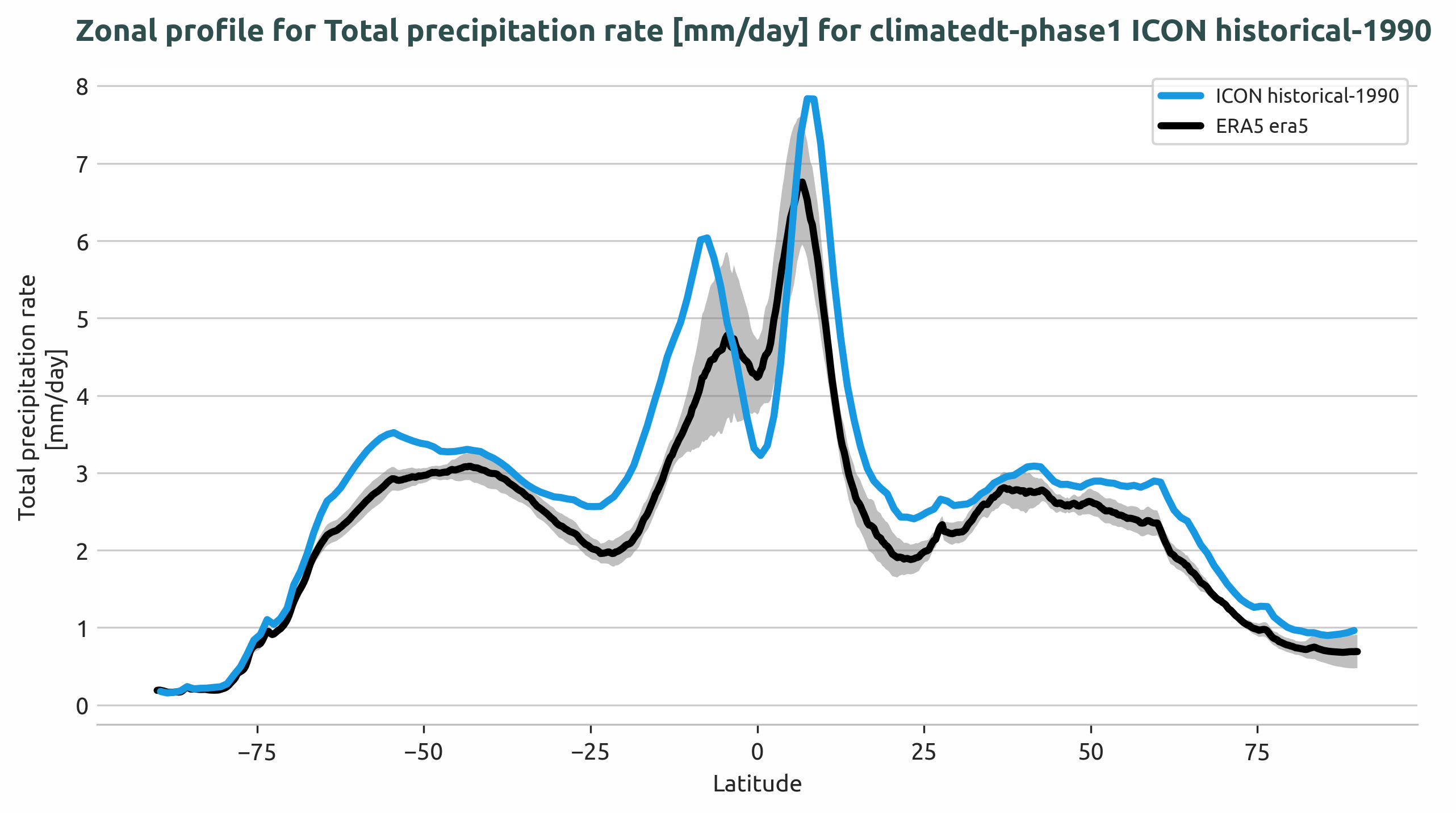
../_images/lat_lon_profiles_zonal_profile_longterm_tprate_Tropics.png — Long-term zonal mean precipitation rate profile for the Tropics region, showing ICON model output compared to ERA5 reference data with ±2σ uncertainty bands.

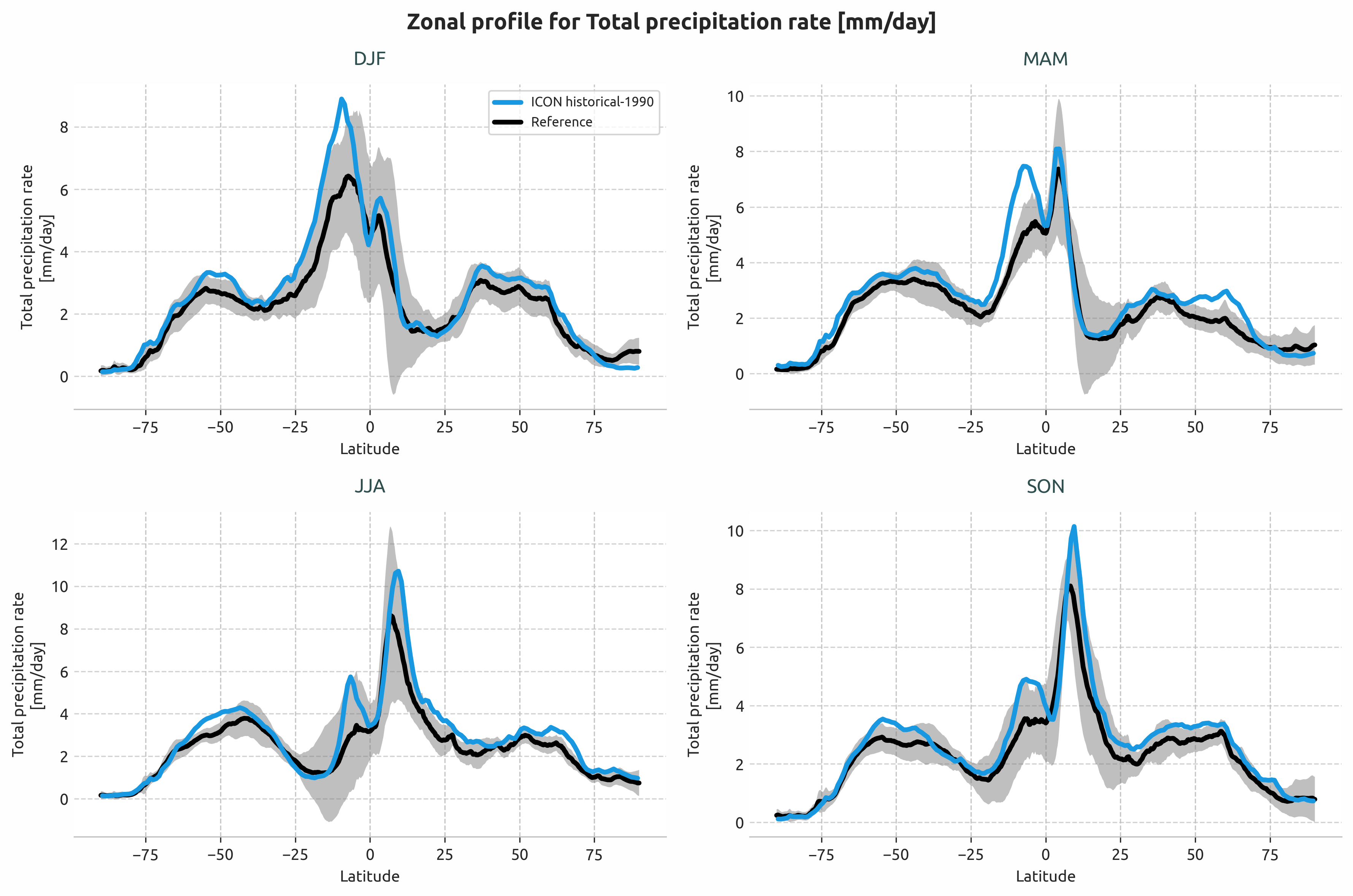
../_images/lat_lon_profiles_zonal_profile_seasonal_tprate_Tropics.png — Seasonal zonal mean precipitation rate profiles (DJF, MAM, JJA, SON) for the Tropics region.

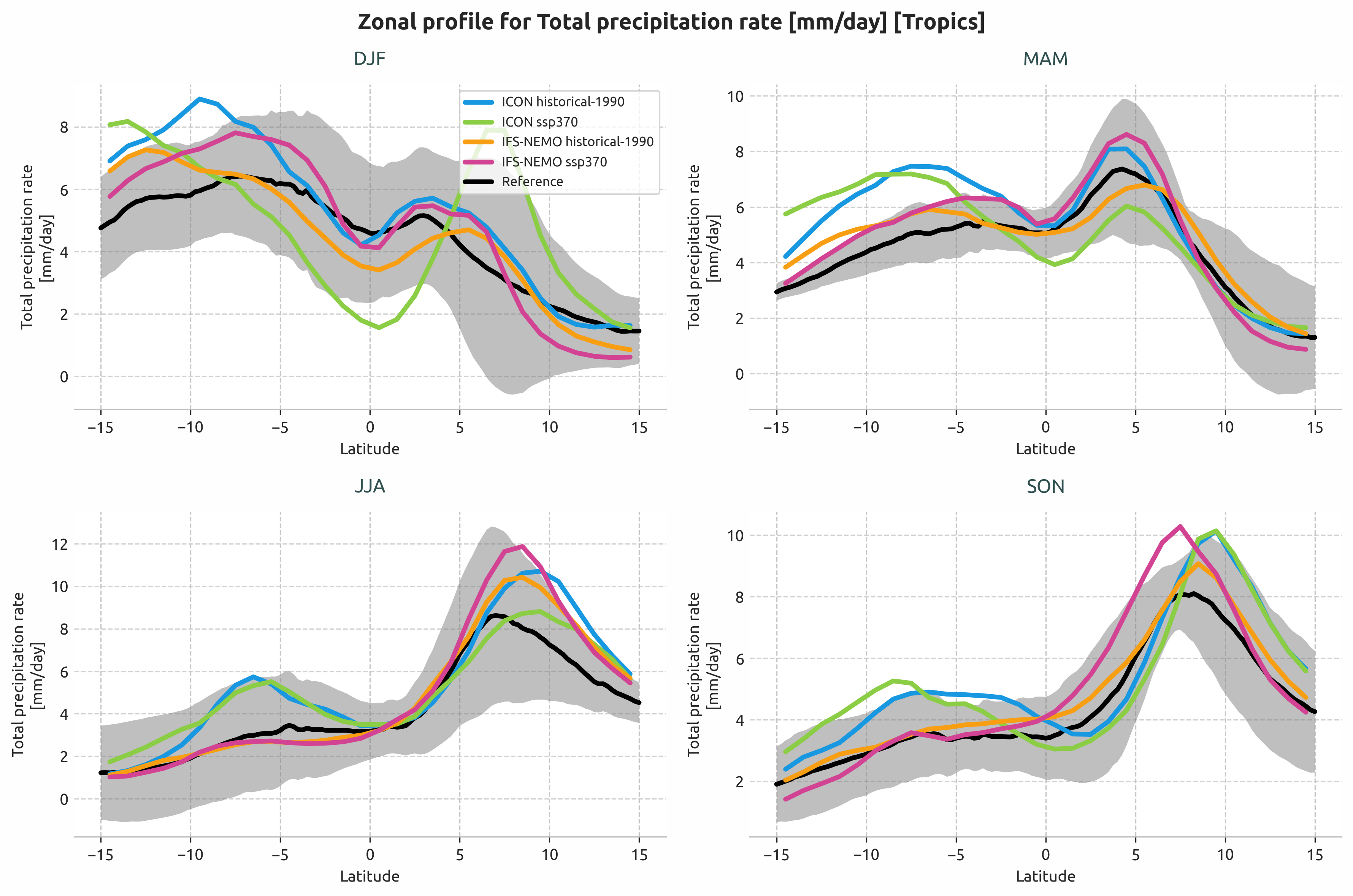
../_images/lat_lon_profiles_zonal_profile_longterm_tprate_Tropics_multimodel.png — Multi-model comparison: ICON and IFS-NEMO historical and SSP3-7.0 scenarios.

Reference datasets

Common reference datasets:

ERA5: ECMWF’s fifth generation reanalysis for global climate
MSWEP: Multi-Source Weighted-Ensemble Precipitation dataset
BERKELEY-EARTH: Berkeley Earth Surface Temperature dataset

Standard deviation can be computed over a custom period using std_startdate and std_enddate to provide ±2σ uncertainty bands in plots.

Authors and contributors

This diagnostic is maintained by Marco Cadau (@mcadau, marco.cadau@polito.it), member of the AQUA team.

Contributions are welcome — please open an issue or pull request. For questions, contact the AQUA team or the maintainers.

Developer Notes

Internal structure:

The diagnostic uses a two-step averaging process:

Spatial averaging via reader.fldmean() with dims parameter:
- Zonal means: dims=['lon'] → latitude profiles
- Meridional means: dims=['lat'] → longitude profiles
Temporal averaging via reader.timmean() with frequency:
- Seasonal: freq='seasonal' → 4 DataArrays [DJF, MAM, JJA, SON]
- Long-term: freq=None → single temporally-averaged DataArray

Data attributes:

Metadata attached to DataArrays for downstream plotting:

AQUA_mean_type: 'zonal' or 'meridional'
AQUA_region: Selected region name
Standard CF attributes: long_name, standard_name, units

Graphics functions:

plot_lat_lon_profiles(): Single-panel line plots
- Handles single or multiple DataArrays
- Supports reference data with optional std shading
- Auto-detects coordinate names (lat/lon, latitude/longitude)
plot_seasonal_lat_lon_profiles(): 4-panel seasonal plots
- Requires exactly 4 elements [DJF, MAM, JJA, SON]
- Each panel supports multiple model lines
- Reference data and std shading per season

Data flow:

LatLonProfiles.retrieve() → Get data from catalog
LatLonProfiles.compute_dim_mean() → Spatial + temporal averaging
LatLonProfiles.compute_std() → Optional std computation
LatLonProfiles.save_netcdf() → Save processed data
PlotLatLonProfiles.__init__() → Load data and metadata
PlotLatLonProfiles.run() → Create and save plots

PlotLatLonProfiles data_type parameter:

data_type='longterm': Single DataArray or list → single-panel plot
data_type='seasonal': List of 4 elements → 4-panel plot

For seasonal plots with multiple models:

data = [
    [model1_DJF, model2_DJF, ...],  # DJF panel
    [model1_MAM, model2_MAM, ...],  # MAM panel
    [model1_JJA, model2_JJA, ...],  # JJA panel
    [model1_SON, model2_SON, ...]   # SON panel
]

API Reference

class aqua.diagnostics.lat_lon_profiles.LatLonProfiles(model: str, exp: str, source: str, catalog: str = None, regrid: str = None, startdate: str = None, enddate: str = None, std_startdate: str = None, std_enddate: str = None, region: str = None, lon_limits: list = None, lat_limits: list = None, regions_file_path: str = None, mean_type: str = 'zonal', diagnostic_name: str = 'latlonprofile', loglevel: str = 'WARNING')

Bases: Diagnostic

Class to compute lat-lon profiles of a variable over a specified region. It retrieves the data from the catalog, computes the mean and standard deviation over the specified period and saves the results to netcdf files.

Supported Frequencies:

‘seasonal’: Computes seasonal means (DJF, MAM, JJA, SON)

‘longterm’: Computes the temporal mean over the entire analysis period

Supported Mean Types:

‘zonal’: Average over longitude, producing latitude profiles
‘meridional’: Average over latitude, producing longitude profilesThe class evaluates a seasonal frequency and the entire period (longterm).

Initialize the LatLonProfiles class.

Parameters:

model (str) – The model to be used for the retrieval of the data.
exp (str) – The experiment to be used for the retrieval of the data.
source (str) – The source to be used for the retrieval of the data.
catalog (str, optional) – The catalog to be used for the retrieval of the data.
regrid (str, optional) – The regridding method to be used for the retrieval of the data.
startdate (str, optional) – The start date of the data to be retrieved.
enddate (str, optional) – The end date of the data to be retrieved.
std_startdate (str, optional) – The start date of the standard deviation period.
std_enddate (str, optional) – The end date of the standard deviation period.
region (str, optional) – The region to be used for the retrieval of the data.
lon_limits (list, optional) – The longitude limits of the region.
lat_limits (list, optional) – The latitude limits of the region.
regions_file_path (str, optional) – The path to the regions file. Default is the AQUA config path.
mean_type (str, optional) – The type of mean to compute (‘zonal’ or ‘meridional’).
diagnostic_name (str, optional) – The name of the diagnostic.
loglevel (str, optional) – The log level to be used for the logging.

compute_dim_mean(freq: str, exclude_incomplete: bool = True, center_time: bool = True, box_brd: bool = True)

Compute the mean of the data. Support for seasonal and longterm means.

Parameters:

freq (str) – The frequency to be used (‘seasonal’ or ‘longterm’).
exclude_incomplete (bool) – If True, exclude incomplete periods.
center_time (bool) – If True, the time will be centered.
box_brd (bool,opt) – choose if coordinates are comprised or not in area selection. Default is True

compute_std(freq: str, exclude_incomplete: bool = True, center_time: bool = True, box_brd: bool = True)

Compute the standard deviation of the data. Support for seasonal and longterm frequencies.

Parameters:

freq (str) – The frequency to be used (‘seasonal’ or ‘longterm’).
exclude_incomplete (bool) – If True, exclude incomplete periods.
center_time (bool) – If True, the time will be centered.
box_brd (bool,opt) – choose if coordinates are comprised or not in area selection. Default is True

retrieve(var: str, formula: bool = False, long_name: str = None, units: str = None, standard_name: str = None, reader_kwargs: dict = {})

Retrieve the data for the specified variable and apply any formula if required.

Parameters:

var (str) – The variable to be retrieved.
formula (bool) – Whether to use a formula for the variable.
long_name (str) – The long name of the variable.
units (str) – The units of the variable.
standard_name (str) – The standard name of the variable.
reader_kwargs (dict) – Additional keyword arguments for the Reader. Default is an empty dictionary.

run(var: str, formula: bool = False, long_name: str = None, units: str = None, standard_name: str = None, std: bool = False, freq: list = ['seasonal', 'longterm'], exclude_incomplete: bool = True, center_time: bool = True, box_brd: bool = True, outputdir: str = './', rebuild: bool = True, reader_kwargs: dict = {})

Run all the steps necessary for the computation of the LatLonProfiles.

Parameters:

var (str) – The variable to be retrieved and computed.
formula (bool) – Whether to use a formula for the variable.
long_name (str) – The long name of the variable.
units (str) – The units of the variable.
standard_name (str) – The standard name of the variable.
std (bool) – Whether to compute the standard deviation.
freq (list) – The frequencies to compute. Options: - ‘seasonal’: Seasonal means (DJF, MAM, JJA, SON) - ‘longterm’: Long-term mean over the entire analysis period
exclude_incomplete (bool) – Whether to exclude incomplete time periods.
center_time (bool) – Whether to center the time coordinate.
box_brd (bool) – Whether to include the box boundaries.
outputdir (str) – The output directory to save the results.
rebuild (bool) – Whether to rebuild existing files.
reader_kwargs (dict) – Additional keyword arguments for the Reader. Default is an empty dictionary.

save_netcdf(freq: str, outputdir: str = './', rebuild: bool = True)

Save the data to a netcdf file.

Parameters:

freq (str) – The frequency of the data (‘seasonal’ or ‘longterm’).
outputdir (str) – The directory to save the data.
rebuild (bool) – If True, rebuild the data from the original files.

class aqua.diagnostics.lat_lon_profiles.PlotLatLonProfiles(data=None, ref_data=None, data_type='longterm', ref_std_data=None, diagnostic_name='lat_lon_profiles', loglevel: str = 'WARNING')

Bases: object

Class for plotting Lat-Lon Profiles diagnostics. This class provides methods to set data labels, description, title, and to plot the data. It handles data arrays regardless of their original temporal frequency, as temporal averaging is handled upstream.

Initialise the PlotLatLonProfiles class. This class is used to plot lat lon profiles data previously processed by the LatLonProfiles class.

Parameters:

data – Can be either: - List of temporally-averaged data arrays for annual plots - List of seasonal data [DJF, MAM, JJA, SON] for seasonal plots
ref_data – Reference data (structure matches data based on data_type)
data_type (str) – ‘longterm’ for single/multi-line longterm plots, ‘seasonal’ for 4-panel seasonal plots
ref_std_data – Reference standard deviation data
diagnostic_name (str) – Name of the diagnostic. Default is ‘lat_lon_profiles’.
loglevel (str) – Logging level. Default is ‘WARNING’.

Note

data_type determines how ‘data’ is interpreted: - ‘longterm’: data should be list of DataArrays for single plot - ‘seasonal’: data should be [DJF, MAM, JJA, SON] for 4-panel seasonal plots

get_data_info(): Extract metadata from data arrays based on data_type.

plot(data_labels=None, ref_label=None, title=None, style=None)

Unified plotting method that handles all plotting scenarios based on data_type.

Parameters:

data_labels (list, optional) – Labels for the data.
ref_label (str, optional) – Label for the reference data.
title (str, optional) – Title for the plot.
style (str, optional) – Plotting style. Default is the AQUA style.

Returns:

Matplotlib figure and axes objects.

Return type:

tuple

plot_seasonal_lines(data_labels=None, title=None, style=None)

Plot seasonal means using plot_seasonal_lat_lon_profiles. Creates a 4-panel plot with DJF, MAM, JJA, SON only.

Parameters:

data_labels (list) – List of data labels.
title (str) – Title of the plot.
style (str) – Plotting style. Default is the AQUA style

Returns:

Figure object. axs (list): List of axes objects.

Return type:

fig (matplotlib.figure.Figure)

run(outputdir='./', rebuild=True, dpi=300, style=None, format='png')

Unified run method that handles all plotting scenarios.

Parameters:

outputdir (str) – Output directory to save the plot.
rebuild (bool) – If True, rebuild the plot even if it already exists.
dpi (int) – Dots per inch for the plot.
style (str) – Plotting style. Default is the AQUA style.
format (str) – Format of the plot (‘png’ or ‘pdf’). Default is ‘png’.

save_plot(fig, description: str = None, rebuild: bool = True, outputdir: str = './', dpi: int = 300, format: str = 'png', diagnostic: str = None)

Save the plot to a file.

Parameters:

fig (matplotlib.figure.Figure) – Figure object.
description (str) – Description of the plot.
rebuild (bool) – If True, rebuild the plot even if it already exists.
outputdir (str) – Output directory to save the plot.
dpi (int) – Dots per inch for the plot.
format (str) – Format of the plot (‘png’ or ‘pdf’). Default is ‘png’.
diagnostic (str) – Diagnostic name to be used in the filename as diagnostic_product.

set_data_labels(): Set the data labels for the plot based on data_type.

set_description(): Set the caption for the plot. Specialized for Lat-Lon Profiles diagnostic.

set_ref_label()

Set the reference label for the plot. The label is extracted from the reference data array attributes.

Returns:: Reference label for the plot.
Return type:: ref_label (str)

set_title()

Set the title for the plot. Specialized for Lat-Lon Profiles diagnostic.

Returns:: Title for the plot.
Return type:: title (str)