Global Biases Diagnostic
Description
The GlobalBiases class is a tool for analyzing and visualizing 2D biases between two datasets. It enables a comparative analysis where one dataset is treated as the reference, often observational data like ERA5. However, it can also be used to compare two model datasets, making it suitable for examining differences between historical and scenario experiments.
This class provides functionality for bias analysis, including the ability to: - Plot bias maps to visualize spatial variations. - Analyze seasonal variations in biases. - Generate vertical profiles to assess biases across pressure levels.
Structure
global_biases.py: contains the GlobalBiases classcli_global_biases.py: the command line interface (CLI) script to run the diagnostic.
Input variables
The diagnostic requires the variables that the user wants to analyse.
A list of the variables that are compared automatically when running the full diagnostic is provided in the configuration files
available in the config/diagnostics/global_biases directory.
Some of the variables that are tipically used in this diagnostic are:
2m temperature (2t)
Total Precipitation (tprate)
Zonal and meridional wind (u, v)
Specific humidity (q)
The data we retrieve through the provided functions have monthly timesteps and a 1x1 deg resolution via the Low Resolution Archive. A higher resolution is not necessary for this diagnostic.
Basic usage
The basic usage of this diagnostic is explained with a working example in the notebook provided in the notebooks/diagnostics/global_biases directory.
The basic structure of the analysis is the following:
from aqua import Reader
from aqua.diagnostics import GlobalBiases

#define and retrieve the data to use for the analysis
reader_ifs_nemo = Reader(model = 'IFS-NEMO', exp = 'historical-1990', source = 'lra-r100-monthly')
data_ifs_nemo = reader_ifs_nemo.retrieve()

reader_era5 = Reader(model="ERA5", exp="era5", source="monthly")
data_era5 = reader_era5.retrieve()

global_biases = GlobalBiases(data=data_ifs_nemo, data_ref=data_era5, var_name='2t', loglevel = 'INFO',
                             model="IFS-NEMO", exp="historical-1990", model_obs="ERA5")

global_biases.plot_bias()
The user can also define the start and end date of the analysis and the reference dataset.
Note
A catalogs argument can be passed to the class to define the catalogs to use for the analysis.
If not provided, the Reader will identify the catalogs to use based on the models, experiments and sources provided.
CLI usage
The diagnostic can be run from the command line interface (CLI) by running the following command:
cd $AQUA/src/aqua_diagnostics/global_biases
python cli_global_biases.py --config_file <path_to_config_file>
Additionally the CLI can be run with the following optional arguments:
--config,-c: Path to the configuration file.--nworkers,-n: Number of workers to use for parallel processing.--loglevel,-l: Logging level. Default isWARNING.--catalog: Catalog to use for the analysis. It can be defined in the config file.--model: Model to analyse. It can be defined in the config file.--exp: Experiment to analyse. It can be defined in the config file.--source: Source to analyse. It can be defined in the config file.--outputdir: Output directory for the plots.--cluster: Dask cluster address.
Config file structure
The configuration file is a YAML file that contains the following information:
dataandobs: dictionaries with the information about the model and reference data to use for the analysis.
data:
  catalog: null
  model: 'IFS-NEMO'
  exp: 'historical-1990'
  source: 'lra-r100-monthly'

obs:
  catalog: null
  model: 'ERA5'
  exp: 'era5'
  source: 'monthly'
output: a block describing the details of the output. Is contains:outputdir: the output directory for the plots.rebuild: a boolean that enables the rebuilding of the plots.filename_keys: a list of keys for constructing the output filenames.save_netcdf: a boolean that enables the saving of the plots in NetCDF format.save_pdf: a boolean that enables the saving of the plots in pdf format.save_png: a boolean that enables the saving of the plots in png format.dpi: the resolution of the plots.
diagnostic_attributes: a block with the following information:variables: the list of variables to analyse.plev: the specific pressure level to analyse (default: null)seasons: a boolean that enables the seasonal analysis.seasons_stat: the statistic to use for the seasonal analysis (e.g., ‘mean’).vertical: a boolean that enables the vertical profiles.regrid: the grid you want your data to be regridded to (e.g. ‘r100’).startdate_data: the start date of the dataset.enddate_data: the end date of the dataset.startdate_obs: the start date of the reference dataset.enddate_obs: the end date of the reference dataset.
biases_plot_params: a block defining colorbar limits for plotting biases. Each variable can have its own range.
Output
The diagnostic generates three types of plots for each variable:
The global bias of the model compared to the reference dataset.
The global bias of the model compared to the reference dataset for each season.
If the variable is 3d, a vertical profile of the bias of the model compared to the reference dataset at each pressure level.
These plots are saved in a PDF and png format as well as NetCDF files.
Observations
The diagnostic uses ERA5 as a default reference dataset for the bias analysis. Custom reference datasets can be used.
Example Plots
All these plots can be produced by running the notebooks in the notebooks directory on LUMI HPC.
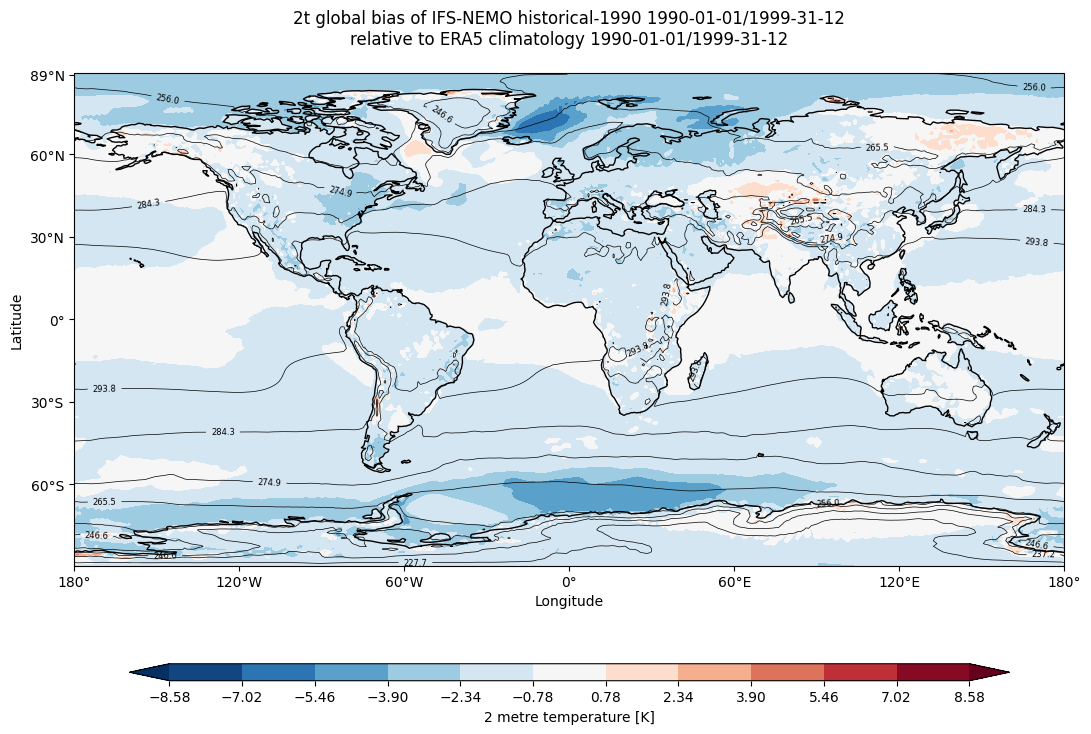
Global mean temperature bias of IFS-NEMO historical-1990 with respect to ERA5 climatology.
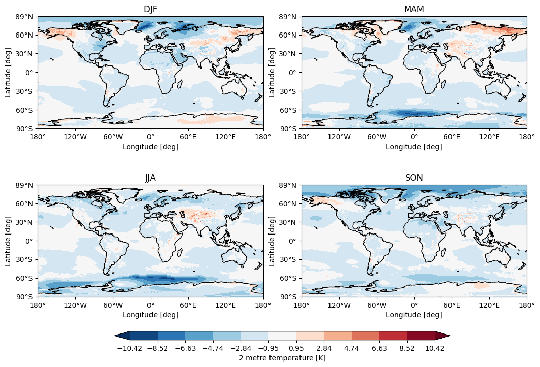
Seasonal temperature bias of IFS-NEMO historical-1990 with respect to ERA5 climatology.
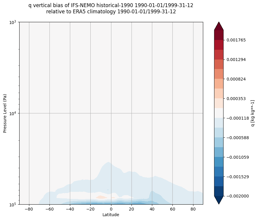
Vertical bias of q of IFS-NEMO historical-1990 with respect to ERA climatology.
Available demo notebooks
Notebooks are stored in diagnostics/global_biases/notebooks:
Detailed API
This section provides a detailed reference for the Application Programming Interface (API) of the timeseries diagnostic,
produced from the diagnostic function docstrings.
- class aqua.diagnostics.global_biases.GlobalBiases(data=None, data_ref=None, var_name=None, plev=None, outputdir=None, loglevel='WARNING', model=None, exp=None, startdate_data=None, enddate_data=None, model_obs=None, startdate_obs=None, enddate_obs=None)
Bases:
objectA class to process and visualize global mean data.
- data
Input data for analysis.
- Type:
xr.Dataset
- data_ref
Reference data for comparison.
- Type:
xr.Dataset
- var_name
Name of the variable to analyze.
- Type:
str
- plev
Pressure level to select.
- Type:
float
- outputdir
Directory to save output plots.
- Type:
str
- loglevel
Logging level.
- Type:
str
- model
Model name for labeling.
- Type:
str, optional
- exp
Experiment name for labeling.
- Type:
str, optional
- startdate_data
Start date of data period.
- Type:
str, optional
- enddate_data
End date of data period.
- Type:
str, optional
- model_obs
Obs name for labeling.
- Type:
str, optional
- startdate_obs
Start date of reference period.
- Type:
str, optional
- enddate_obs
End date of reference period.
- Type:
str, optional
- plot_bias(stat='mean', vmin=None, vmax=None)
Plots global biases or a single dataset map if reference data is unavailable.
- Parameters:
stat (str) – Statistic for calculation (‘mean’ by default).
vmin (float, optional) – Minimum colorbar value.
vmax (float, optional) – Maximum colorbar value.
- Returns:
Matplotlib figure, axis objects, and xarray Dataset of the calculated bias if available.
- Return type:
tuple
- plot_seasonal_bias(seasons_stat='mean', vmin=None, vmax=None)
Plots seasonal biases for each season (DJF, MAM, JJA, SON) and returns an xarray.Dataset containing the calculated seasonal biases.
- Parameters:
seasons_stat (str) – Statistic for seasonal analysis (‘mean’ by default).
vmin (float, optional) – Minimum colorbar value.
vmax (float, optional) – Maximum colorbar value.
- Returns:
Matplotlib figure, axis objects, and an xarray.Dataset of the calculated seasonal biases.
- Return type:
tuple
- plot_vertical_bias(data=None, data_ref=None, var_name=None, plev_min=None, plev_max=None, vmin=None, vmax=None)
Calculates and plots the vertical bias between two datasets.
- Parameters:
data (xr.Dataset, optional) – Dataset for analysis.
data_ref (xr.Dataset, optional) – Reference dataset for comparison.
var_name (str, optional) – Variable name to analyze.
plev_min (float, optional) – Minimum pressure level.
plev_max (float, optional) – Maximum pressure level.
vmin (float, optional) – Minimum colorbar value.
vmax (float, optional) – Maximum colorbar value.
- Returns:
Matplotlib figure, axis objects, and xarray Dataset of the calculated bias.
- Return type:
tuple
- static select_pressure_level(data, plev, var_name)
Selects a specified pressure level from the dataset.
- Parameters:
data (xr.Dataset) – Dataset to select from.
plev (float) – Desired pressure level.
var_name (str) – Variable name to filter by.
- Returns:
Filtered dataset at specified pressure level.
- Return type:
xr.Dataset
- Raises:
NoDataError – If specified pressure level is not available.