Ocean3D
Description
This package contains two submodules to monitor and evaluate the 3D ocean evolution and mean state:
Ocean Drifts: to characterize and monitor model drifts.Ocean Circulation: to evaluate the realism of the model in simulating key precursors of the ocean circulation.
All these diagnostics are produced in a consistent way for any selected model simulation. Additionally, there are newly added multi-model diagnostic functions under both submodules that allow the comparison of different experiments at once.
Structure
The ocean3d diagnostic follows a class structure and consists of the following files:
cli: Folder to run the ocean diagnostics from the command line;cli_ocean3d.py: a python file that contains the command line ocean diagnostics;config.yaml: config file containing details for the cli;
configFolder containing necessary information for ocean3d;regions.yaml: yaml file containing the predefined regions where users can also define regions;
notebooks: Folder contains notebooks demonstrating the functions;ocean_drifts.ipynb: an ipython notebook with examples on how to apply the ocean drift diagnostics;ocean_circulation.ipynb: an ipython notebook with examples on how to apply the ocean circulation diagnostics;multi_model_analysis.ipynb: an ipython notebook with examples on how to apply the multi model diagnostics;
ocean3d: Folder containing the ocean3d functions;ocean_circulation: Folder containing the ocean circulation functions;multi_model: Folder containing the ocean circulation functions;mld.py: a python file that contains the functions for mixed layer depth;stratification.py: a python file that contains the functions for stratification;
ocean_drifts: Folder containing the ocean drift functions;multi_model: Folder containing the ocean drift functions;hovmoller_plot.py: a python file that contains the functions for hovmoller plot;time_series.py: a python file that contains the functions for time series;trends.py: a python file that contains the functions for trends;
ocean_utils.py: a python file that contains functions used in both ocean3d diagnostic modules;
README.md: a readme file that contains some technical information on how to install the ocean3d diagnostic and its environment.
Input variables example
avg_thetao(Ocean potential temperature, GRIB paramid 150129)avg_so(Sea water practical salinity, GRIB paramid 151130)
Output
This module exports all the data and diagnostics used to create the different figures except the multi-model diagnostics.
CLI (Command Line Interface)
Under the cli folder, upon updating the config file and running the cli_ocean3d.py, users will generate all the ocean3d diagnostics figures.
python cli_ocean3d.py --model <model> --exp <experiment> --source <source>
Prepare the o3d request
Single Model analysis
ocean3d typical request looks like this, but some details may change depending on the selected function.
Also, the requests for multi-model diagnostics are also different.
We recommend to look into the notebooks to get a clearer idea of function-specific details.
o3d_request= {'model':'IFS-NEMO', 'exp':'historical-1990', 'source': 'lra-r100-monthly',
              'data': data, 'obs_data': obs_data, 'region':'Labrador Sea',
              'latS':None, 'latN':None, 'lonW':None, 'lonE':None,
              'output':True, "time" : "February", 'output_dir':'./output'}
Multi Model analysis
For multi-model analysis, the request looks like this, but some details may change depending on the selected function. We recommend looking into the notebooks to get a clearer idea of function-specific details.
data_dict = {'EN4 1':en4_1, 'EN4 2':en4_2, 'IFS-NEMO Historical':ifs_nemo_historical,
             'IFS-NEMO ssp370':ifs_nemo_ssp370,
             'icon Historical':icon_historical,'icon ssp370': icon_ssp370}
o3d_request= {'data_dict': data_dict,'region':'Labrador Gin Seas',
              'latS':None,'latN':None,'lonW':None,'lonE':None,
              'output':True,"time" : "March",'output_dir':'./output'}
Functions used
Single Model analysis
hovmoller_plot(o3d_request)
hovmoller_lev_time_plot: This function requires the input data and a region of choice. It produces a Hovmöller plot of regionally averaged temperature and salinity including three types of subplots. The region name supports all the major oceans and seas, in case users require a custom region, they can fill in the values of latitude, and longitude in the boxes as desired.
time_series(o3d_request)
time_series: This function requires the input data and a region of choice. It produces time series plots of regionally averaged temperature and salinity including three types of subplots for a predefined or customized list of vertical levels. The region name supports all the major oceans and seas, in case users require a custom region, they can fill in the values of latitude, and longitude in the boxes.
multilevel_trend(o3d_request)
multilevel_trend: This function requires the input data, a region of choice, and (optionally) a choice of depth levels. It produces lon-lat maps of linear temporal trends of temperature and salinity over the selected region for a predefined or customized list of vertical levels. The region name supports all the major oceans and seas, in case users require a custom region, they can fill in the values of latitude, and longitude in the boxes.
zonal_mean_trend_plot(o3d_request)
Zonal Mean Trend Plot: This function requires the input data and a region of choice. It produces plots of zonally averaged linear temporal trends plot of temperature and salinity as a function of depth and latitude. The zonal average is produced over the selected region, whose name supports all the major oceans and seas; in case users require a custom region, they can fill in the values of latitude and longitude in the boxes.
stratification(o3d_request)
Stratification plot: This function requires the input data, a region of choice, and a temporal period to compute the climatology. It produces a stratification plot of Temperature, salinity and Density, including the overlapped data with the observation. The region name supports all the major oceans and seas, in case users require a custom region, they can fill in the values of latitude, and longitude in the boxes.
plot_spatial_mld_clim(o3d_request)
Mixed Layer Depth Plot: This function requires the input data, a region of choice, and a temporal period to compute the climatology. It produces a time series plot of temperature and salinity. Users have the option of choosing whether they want to use the whole obs data or overlapped obs data with the model. The region name supports all the major oceans and seas; in case users require a custom region, they can fill in the values of latitude, and longitude in the boxes.
Multi Model analysis
mld_multi_model(o3d_request)
This function provides the plots for mixed player depth provided the different models or observations and regions.
trend_plot = trend(o3d_request)
trend_plot.plot()
This function provides the plots for trends provided the different models or observations, depth level and regions.
strat = stratification(o3d_request)
strat.plot()
This function provides the plots for stratification (Temperature, salinity, and density profile) provided the different models or observations and regions.
timeser = time_series(o3d_request)
timeser.plot()
This function provides the plots for standardized anomaly time series provided the different models or observations and regions.
Methods used
All regional averages have been produced with area weights.
Temporal trends are computed as linear trends and estimated over the whole temporal span of the dataset.
The mixed layer depth is computed by the function
compute_mld_contfromsigma0monthly fields following the criteria from de Boyer Montegut et al (2004)Density fields are computed from absolute salinity and conservative temperature fields using the TEOS-10 equations.
Absolute salinity and conservative temperature are also computed from practical salinity and potential temperature fields with TEOS-10 equations.
Observations
EN4.2.2.g10 ocpt and so observations for the period 1950-2022
References
de Boyer Montégut, C., Madec, G., Fischer, A. S., Lazar, A., and Iudicone, D. (2004): Mixed layer depth over the global ocean: An examination of profile data and a profile-based climatology. J. Geophys. Res., 109, C12003, doi:10.1029/2004JC002378
Gouretski and Reseghetti (2010): On depth and temperature biases in bathythermograph data: development of a new correction scheme based on analysis of a global ocean database. Deep-Sea Research I, 57, 6. doi: http://dx.doi.org/10.1016/j.dsr.2010.03.011
A code to compute very efficiently the linear trends has been adapted from this website: https://stackoverflow.com/questions/52108417/how-to-apply-linear-regression-to-every-pixel-in-a-large-multi-dimensional-array
Example Plot(s)
Examples showing an individual simulation refer to the IFS-NEMO historical experiment at Tco1279/eORCA12
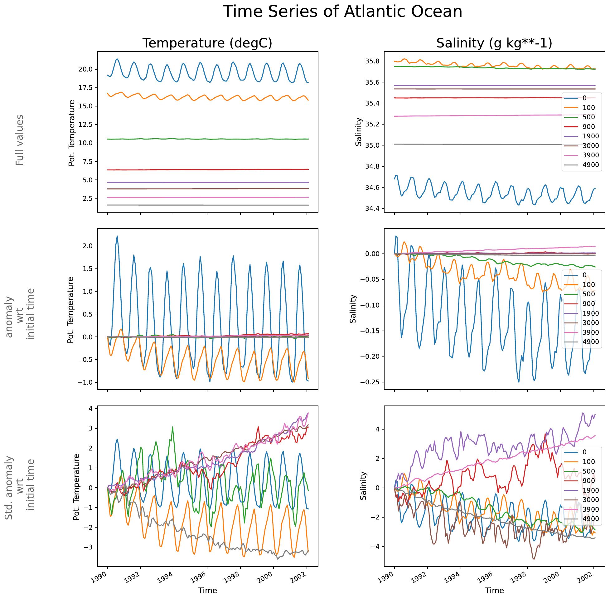
This is an example of the multipanel plots of the spatially averaged T, S timeseries at different levels
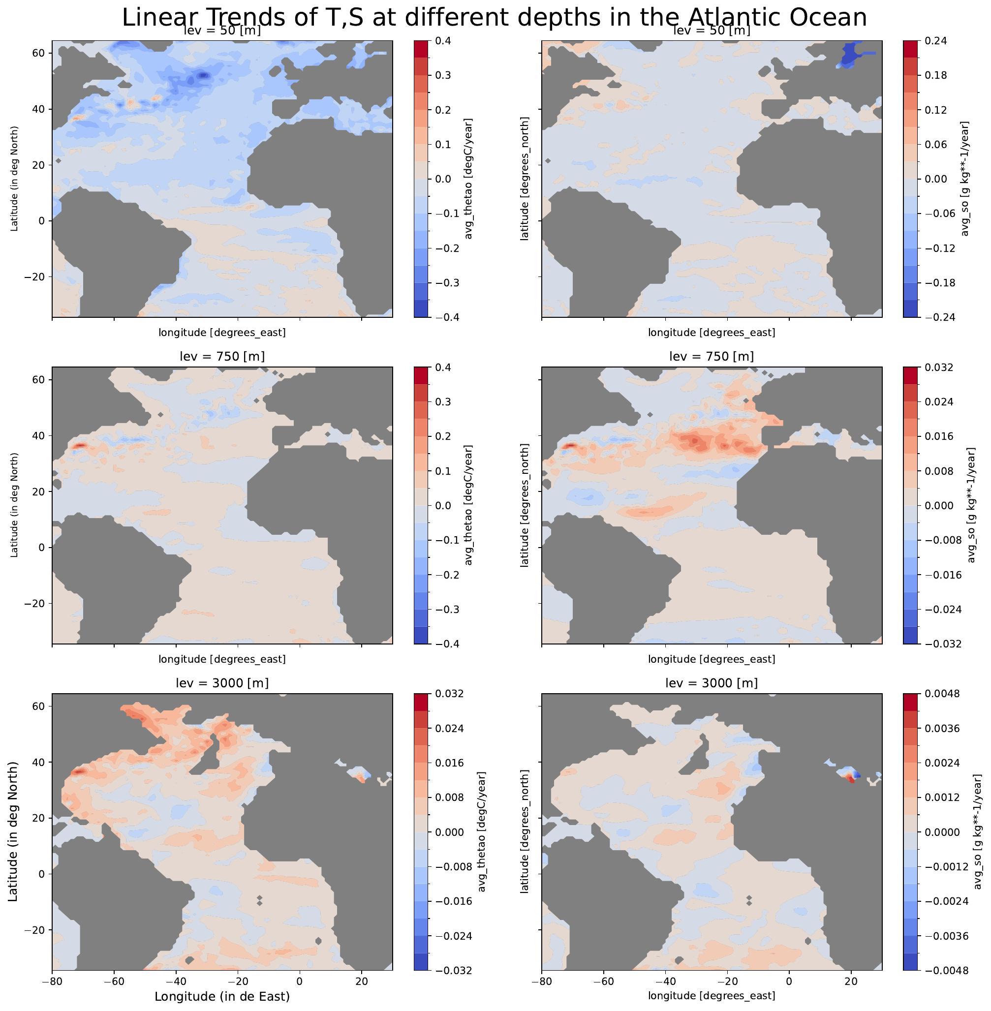
This is an example of the multi-panel plots of lat-lon maps of temporal trends in T, S at different levels
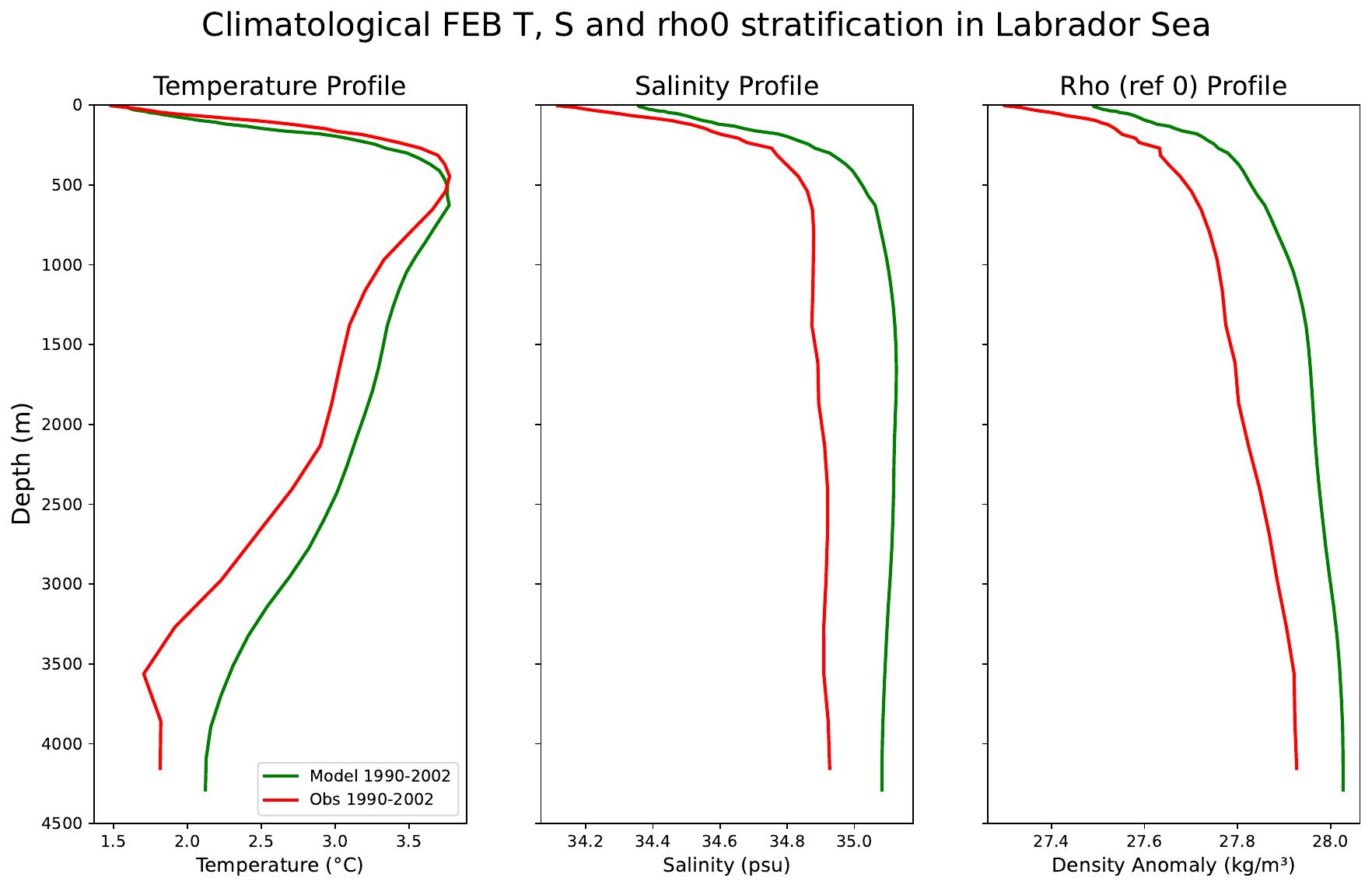
This is an example of one of the climatological stratification profiles.
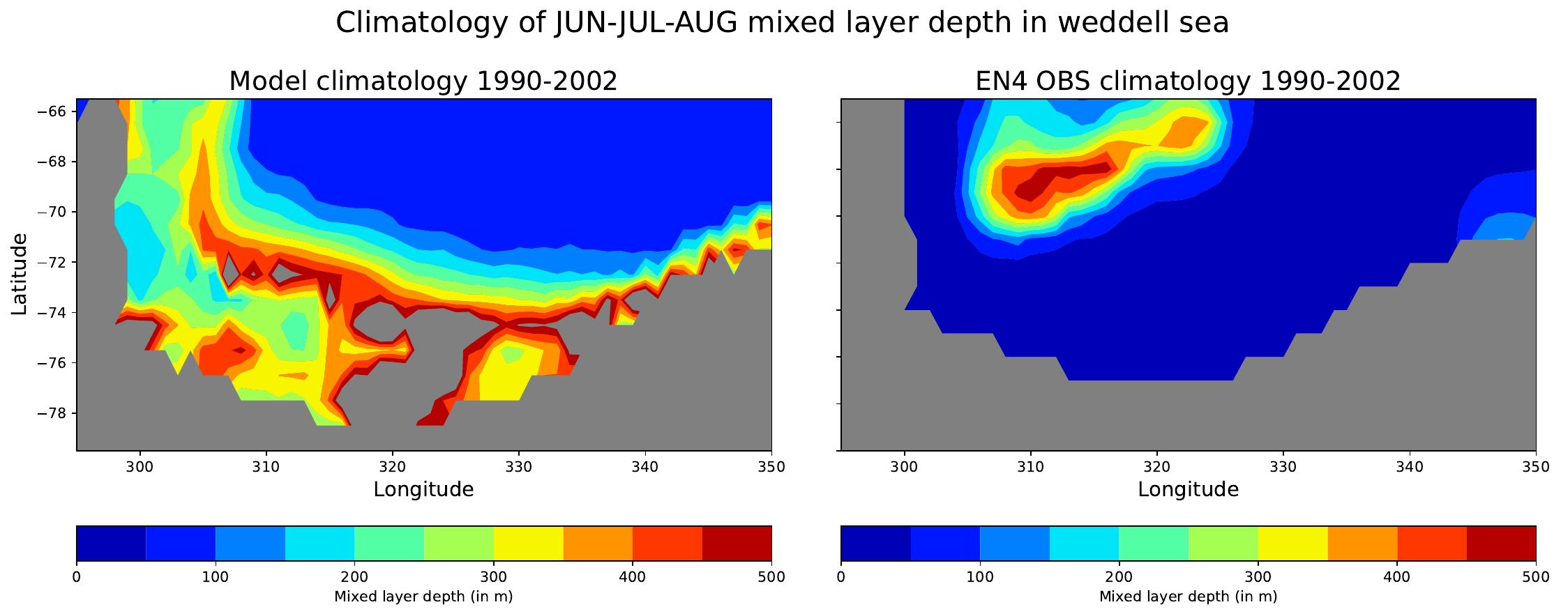
This is an example of one of the mixed-layer depth climatologies. Unit is meter.
This is an example of multi-model time series plot.
This is an example of multi-model surface trends of global ocean.
This is an example of multi-model stratification of two regions.
This is an example of multi-model MLD.
Available demo notebooks
Notebooks are stored in diagnostics/ocean3d/notebooks
Detailed API
This section provides a detailed reference for the Application Programming Interface (API) of the “ocean3d” diagnostic, produced from the diagnostic function docstrings.
Ocean3D module
- class ocean3d.hovmoller_plot(o3d_request)
Bases:
objectA class for generating Hovmoller plots from ocean3d data.
- Parameters:
o3d_request – Request object containing necessary data for plot generation.
- Inherits all attributes from the parent class.
Initializes the hovmoller_plot object.
- Parameters:
o3d_request – Request object containing necessary data for plot generation.
- data_for_hovmoller_lev_time_plot()
Processes data for generating Hovmoller plots.
- Returns:
None
- define_lev_values(data_proc)
Defines the levels for temperature and salinity data.
- Parameters:
data_proc – Processed ocean data.
- Returns:
A tuple containing arrays of temperature levels and salinity levels.
- Return type:
Tuple
- loop_details(i, fig, axs)
Loop over plot details to generate Hovmoller plots.
- Parameters:
i – Index indicating the loop iteration.
fig – Figure object for plotting.
axs – Axes object for plotting.
- plot()
Generate and display time series plots.
- Returns:
None
- class ocean3d.time_series(o3d_request)
Bases:
hovmoller_plotA class for generating time series plots from ocean3d data.
Inherits from hovmoller_plot.
- Parameters:
o3d_request – Request object containing necessary data for plot generation.
- Inherits all attributes from the parent class.
Initializes the time_series object.
- Parameters:
o3d_request – Request object containing necessary data for plot generation.
- loop_details(i, fig, axs)
Loop over plot details to generate time series plots.
- Parameters:
i – Index indicating the loop iteration.
fig – Figure object for plotting.
axs – Axes object for plotting.
- plot()
Generate and display time series plots.
- Returns:
None