Other core functionalities

Time Statistics

Input data may not be available at the desired time frequency. It is possible to perform time statistics, including time averaging, minimum, maximum and standard deviation at a given time frequency by using the timstat() method and its sibilings timmean(), timmin(), timmax() and timstd().

reader = Reader(model="IFS", exp="tco2559-ng5", source="ICMGG_atm2d")
data = reader.retrieve()
daily = reader.timmean(data, freq='daily')
# alternatively: daily = reader.timstat(data, stat='mean', freq='daily')

Data have now been averaged at the desired daily timescale. Similarly operations can be performed with others methods.

Warning

If you do not specify the freq argument, the statistical operation will be operated on the entire dataset!

Some extra options are available:

• exclude_incomplete=True: this flag will remove averaged chunks which are not complete (for example, verify that all the record from each month are available before doing the time mean).

• center_time=True: this flag will center the time coordinate on the mean time window.

• time_bounds=True: this flag can be activated to build time bounds in a similar way to CMOR-like standard.

Detrending

For some analysis, removing from the data a linear trend can be helpful to highlight the internal variability. The detrend method can be used as a high-level wrapper of xarray functionalities to achieve this goal.

reader = Reader(model="IFS", exp="tco2559-ng5", source="ICMGG_atm2d")
data = reader.retrieve()
daily = reader.detrend(data['2t'], dim='time')

In this way, linear trend is removed from each grid point of the original dataset along the time dimension. Other dimension can be targeted too, although with limited physical meaning. Of course, it can be used in collaboration with temporal and spatial averaging. Higher order polynominial fits are available too.

Some options includes:

• degree: this will define with an integer the order of the polynominial fit. Default is 1, i.e. linear detrending.

• skipna=True: removing the NaN from the fit. Default is True.

Warning

Detrending might lead to incorrect results if there is not an equal amount of time elements (e.g. same amount of months or days) in the dataset.

Spatial Averaging

When we instantiate the Reader object, grid areas for the source files are computed if not already available. After this, we can use them for spatial averaging using the fldmean() method, obtaining time series of global (field) averages. For example, if we run the following commands:

tprate = data.tprate
global_mean = reader.fldmean(tprate)

we get a time series of the global average tprate.

It is also possible to apply a regional section to the domain before performing the averaging:

tprate = data.tprate
global_mean = reader.fldmean(tprate, lon_limits=[-50, 50], lat_limits=[-10,20])

Warning

In order to apply an area selection the data Xarray must include lon and lat as coordinates. It can work also on unstructured grids, but information on coordinates must be available. If the dataset does not include these coordinates, this can be achieved with the fixer described in the Fixer functionalities section.

Time selection

Even if slicing your data after the retrieve() method is an easy task, being able to perform a time selecetion during the Reader initialization can speed up your code, having less metadata to explore. For this reason startdate and enddate options are available both during the Reader initialization and the retrieve() method to subselect immediatly only a chunck of data.

Note

If you’re streaming data check the section Streaming of data to have an overview of the behaviour of the Reader with these options.

Level selection

Similarly to Time selection, level selection is a trivial operation, but when dealing with high-resolution 3D datasets, only ask for the required levels can speed up the retrieve process.

When reading 3D data it is possible to specify already during retrieve() which levels to select using the level keyword. The levels are specified in the same units as they are stored in the archive (for example in hPa for atmospheric IFS data, but an index for NEMO data in the FDB archive).

Note

In the case of FDB data this presents the great advantage that a significantly reduced request will be read from the FDB (by default all levels would be read for each timestep even if later a sel() or isel() selection is performed on the XArray).

Warning

If you’re dealing with level selection and regridding, please take a look at the section Level selection and regridding.

Streaming of data

The Reader class includes the ability to simulate data streaming to retrieve chunks of data of a specific time length.

Basic usage

To activate the streaming mode the user should specify the argument streaming=True in the Reader initialization. The user can also choose the length of the data chunk with the aggregation keyword (e.g. in pandas notation, or with aliases as daily, monthly etc. or days, months etc.). The default is S (step), i.e. single saved timesteps are read at each iteration. The user can also specify the desired initial and final dates with the keywords startdate and enddate.

If, for example, we want to stream the data every three days from '2020-05-01', we need to call:

reader = Reader(model="IFS", exp= "tco2559-ng5", source="ICMGG_atm2d",
                streaming=True, aggregation = '3D', startdate = '2020-05-01')
data = reader.retrieve()

The data available with the first retrieve will be only 3 days of the available times. The retrieve() method can then be called multiple times, returning a new chunk of 3 days of data, until all data are streamed. The function will automatically determine the appropriate start and end points for each chunk based on the internal state of the streaming process.

If we want to reset the state of the streaming process, we can call the reset_stream() method.

Iterator streaming

Another possibility to deal with data streaming is to use the argument stream_generator=True in the Reader initialization:

reader = Reader(model="IFS", exp= "tco2559-ng5", source="ICMGG_atm2d",
                stream_generator = 'True', aggregation = 'monthly')
data_gen = reader.retrieve()

data_gen is now a generator object that yields the requested one-month-long chunks of data (See Iterator access to data for more info). We can do operations with them by iterating on the generator object like:

for data in data_gen:
    # Do something with the data

Accessors

AQUA also provides a special aqua accessor to Xarray which allows to call most functions and methods of the reader class as if they were methods of a DataArray or Dataset.

Basic usage

Reader methods like reader.regrid() or functions like plot_single_map() can now also be accessed by appending the suffix aqua to a DataArray or Dataset, followed by the function of interest, like in data.aqua.regrid().

This means that instead of writing:

reader.fldmean(reader.timmean(data.tcc, freq="Y"))

we can write:

data.tcc.aqua.timmean(freq="Y").aqua.fldmean()

Note

The accessor always assumes that the Reader instance to be used is either the one with which a Dataset was created or, for new derived objects and for DataArrays of a Datasets, the last instantiated Reader or the last use of the retrieve() method. This means that if more than one reader instance is used (for example to compare different datasets) we recommend not to use the accessor.

Usage with multiple Reader instances

As an alternative the Reader class contains a special set_default() method which sets that reader as an accessor default in the following. The accessor itself also has a set_default() method (accepting a reader instance as an argument) which sets the default and returns the same object.

Usage examples when multiple readers are used:

from aqua import Reader
reader1=Reader(model="IFS", exp="test-tco79", source="short", regrid="r100")  # the default is now reader1
reader2=Reader(model="IFS", exp="test-tco79", source="short", regrid="r200")  # the default is now reader2
data1 = reader1.retrieve()  # the default is now reader1
data2 = reader2.retrieve()  # the default is now reader2
reader1.set_default()  # the default is now reader1
data1r = data1.aqua.regrid()
data2r = data2.aqua.regrid()  # data2 was created by retrieve(), so it remembers its default reader
data2r = data2['2t'].aqua.set_default(reader2).aqua.regrid()  # the default is set to reader2 before using a method

Parallel Processing

Since most of the objects in AQUA are based on xarray, you can use parallel processing capabilities provided by xarray through integration with dask to speed up the execution of data processing tasks.

For example, if you are working with AQUA interactively in a Jupyter Notebook, you can start a dask cluster to parallelize your computations.

from dask.distributed import Client
import dask
dask.config.config.get('distributed').get('dashboard').update({'link':'{JUPYTERHUB_SERVICE_PREFIX}/proxy/{port}/status'})

client = Client(n_workers=40, threads_per_worker=1, memory_limit='5GB')
client

The above code will start a dask cluster with 40 workers and one thread per worker.

AQUA also provides a simple way to move the computation done by dask to a compute node on your HPC system. The description of this feature is provided in the section Slurm utilities.

Graphic tools

The aqua.graphics module provides a set of simple functions to easily plot the result of analysis done within AQUA.

Single map

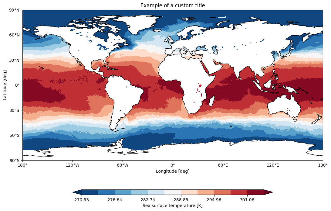
A function called plot_single_map() is provided with many options to customize the plot.

The function takes as input an xarray.DataArray, with a single timestep to be selected before calling the function. The function will then plot the map of the variable and, if no other option is provided, will adapt colorbar, title and labels to the attributes of the input DataArray.

In the following example we plot an sst map from the first timestep of ERA5 reanalysis:

from aqua import Reader, plot_single_map

reader = Reader(model='ERA5', exp='era5', source='monthly')
sst = reader.retrieve(var=["sst"])
sst_plot = sst["sst"].isel(time=0)

plot_single_map(sst_plot, title="Example of a custom title", filename="example",
                outputdir=".", format="png", dpi=300, save=True)

This will produce the following plot:

Single map with differences

A function called plot_single_map_diff() is provided with many options to customize the plot.

The function is built as an expansion of the plot_single_map() function, so that arguments and options are similar. The function takes as input two xarray.DataArray, with a single timestep.

The function will plot as colormap or contour filled map the difference between the two input DataArray (the first one minus the second one). Additionally a contour line map is plotted with the first input DataArray, to show the original data.

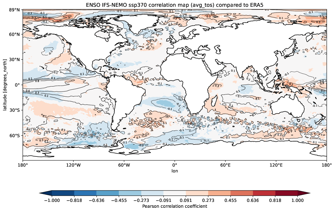
Example of a plot_single_map_diff() output done with the Teleconnections diagnostic. The map shows the correlation for the ENSO teleconnection between IFS-NEMO scenario run and ERA5 reanalysis.

Time series

A function called plot_timeseries() is provided with many options to customize the plot. The function is built to plot time series of a single variable, with the possibility to plot multiple lines for different models and a special line for a reference dataset. The reference dataset can have a representation of the uncertainty over time.

By default the function is built to be able to plot monthly and yearly time series, as required by the Timeseries diagnostic.

The function takes as data input:

• monthly_data: a (list of) xarray.DataArray, each one representing the monthly time series of a model.

• annual_data: a (list of) xarray.DataArray, each one representing the annual time series of a model.

• ref_monthly_data: a xarray.DataArray representing the monthly time series of the reference dataset.

• ref_annual_data: a xarray.DataArray representing the annual time series of the reference dataset.

• std_monthly_data: a xarray.DataArray representing the monthly values of the standard deviation of the reference dataset.

• std_annual_data: a xarray.DataArray representing the annual values of the standard deviation of the reference dataset.

The function will automatically plot what is available, so it is possible to plot only monthly or only yearly time series, with or without a reference dataset.

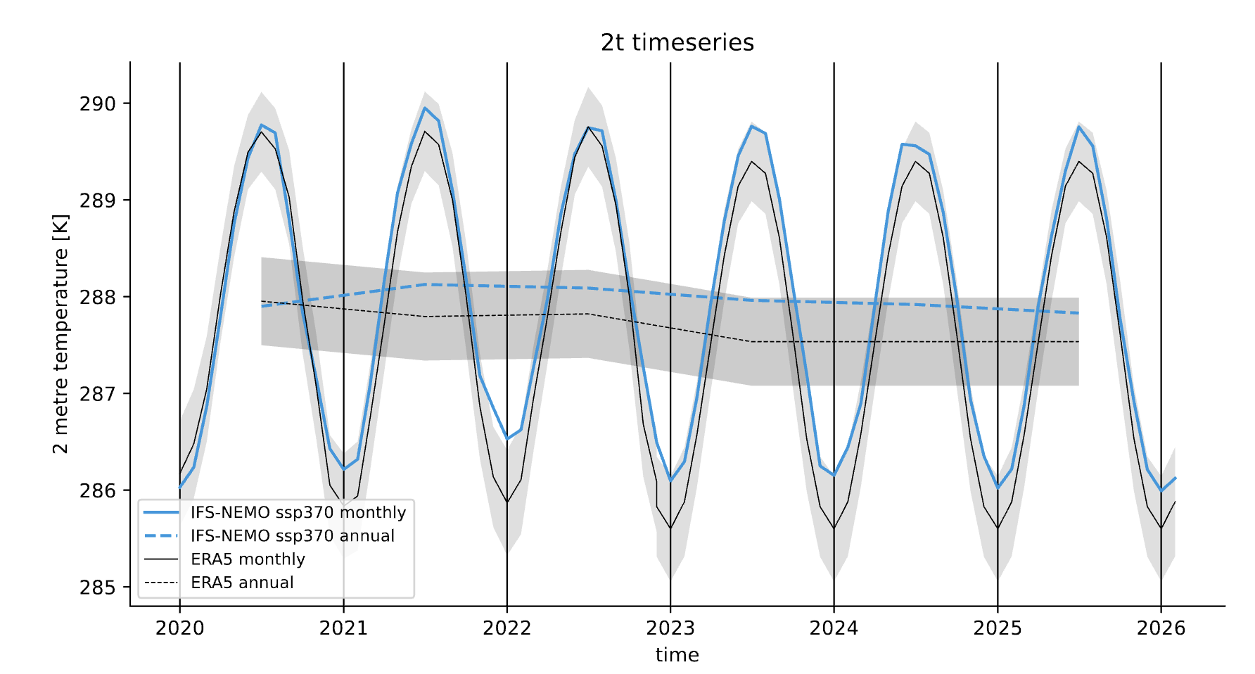
Example of a plot_timeseries() output done with the Timeseries. The plot shows the global mean 2 meters temperature time series for the IFS-NEMO scenario and the ERA5 reference dataset.

Seasonal cycle

A function called plot_seasonalcycle() is provided with many options to customize the plot.

The function takes as data input:

• data: a xarray.DataArray representing the seasonal cycle of a variable.

• ref_data: a xarray.DataArray representing the seasonal cycle of the reference dataset.

• std_data: a xarray.DataArray representing the standard deviation of the seasonal cycle of the reference dataset.

The function will automatically plot what is available, so it is possible to plot only the seasonal cycle, with or without a reference dataset.

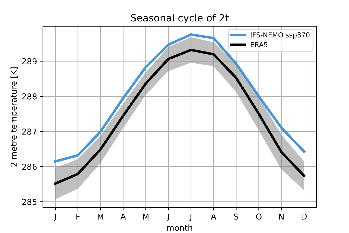
Example of a plot_seasonalcycle() output done with the Timeseries. The plot shows the seasonal cycle of the 2 meters temperature for the IFS-NEMO scenario and the ERA5 reference dataset.

Multiple maps

A function called plot_maps() is provided with many options to customize the plot. The function takes as input a list of xarray.DataArray, each one representing a map. It is built to plot multiple maps in a single figure, with a shared colorbar. This can be userdefined or evaluated automatically. Figsize can be adapted and the number of plots and their position is automatically evaluated.

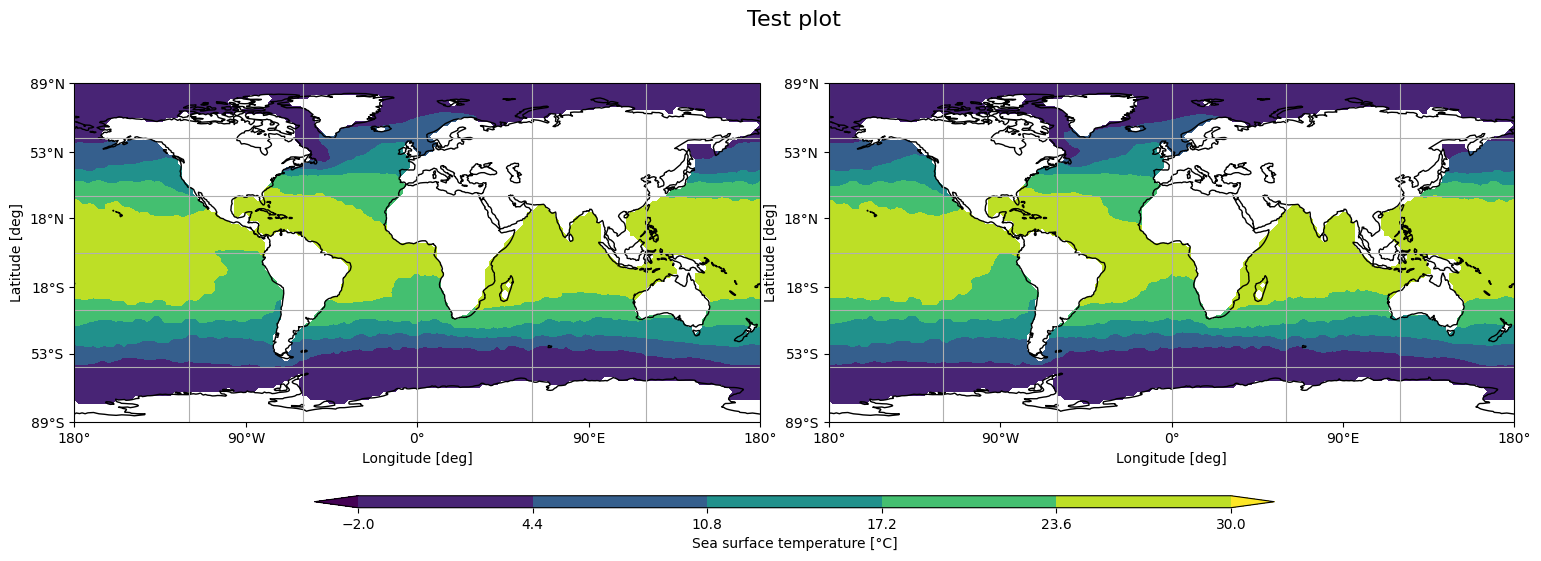
Example of a plot_maps() output.