Timeseries
Description
The diagnostic is composed of three main functionalities that are implemented as three classes:
Timeseries: a class that computes the global mean time series of a given variable or formula for a given model or list of models. Comparison with a reference dataset is also possible.
GregoryPlot: a class that computes the Gregory-like plot for a given model or list of models. Comparison with a reference dataset is also possible.
SeasonalCycle: a class that computes the seasonal cycle of a given variable or formula for a given model or list of models. Comparison with a reference dataset is also possible.
Structure
README.md: a readme file which contains some technical information on how to install the diagnostic and its environment.cli_timeseries.py: the command line interface (CLI) script to run the diagnostic.gregory.py: contains the GregoryPlot class.reference_data.py: contains the code to retrieve the reference data for all the classes.seasonalcycle.py: contains the SeasonalCycle class.timeseries.py: contains the Timeseries class.util.py: contains the utility functions used by the classes.
Input variables
The diagnostic requires the variables that the user wants to analyse.
A list of the variables that are compared automatically when running the full diagnostic is provided in the configuration files
available in the config/diagnostics/timeseries directory.
For the Gregory-like plot, the following variables are required:
2t(2 metre temperature, GRIB paramid 167)mtnlwrf(Mean top net long-wave radiation flux, GRIB paramid 235040)mtnswrf(Mean top net short-wave radiation flux, GRIB paramid 235039)
Basic usage
The basic usage of each class is explained with a working example in the notebooks provided in the notebooks/diagnostics/timeseries directory.
The basic structure of the analysis is the following:
from aqua.diagnostic.timeseries import Timeseries

# Define the models to analyse
models = ['IFS-NEMO', 'ICON']
exps = ['historical-1990', 'ssp370']
sources = ['lra-r100-monthly', 'lra-r100-monthly']

ts = Timeseries(var='2t', models=models, exps=exps, sources=sources,
                startdate='1990-01-01', enddate='1999-12-31',
                std_startdate='1990-01-01', std_enddate='1999-12-31',
                loglevel='INFO')
ts.run()
The same structure can be used for the other classes. As can be seen, more than one model can be analysed at the same time. The user can also define the start and end date of the analysis and the reference dataset.
Note
A catalogs argument can be passed to the class to define the catalogs to use for the analysis.
If not provided, the Reader will identify the catalogs to use based on the models, experiments and sources provided.
CLI usage
The diagnostic can be run from the command line interface (CLI) by running the following command:
cd $AQUA/src/aqua_diagnostics/timeseries
python cli_timeseries.py --config_file <path_to_config_file>
Three configuration files are provided and run when executing the aqua-analysis (see AQUA analysis wrapper). Two configuration files are for atmospheric and oceanic timeseries and gregory plots, and the third one is for the seasonal cycles.
Additionally the CLI can be run with the following optional arguments:
--config,-c: Path to the configuration file.--nworkers,-n: Number of workers to use for parallel processing.--loglevel,-l: Logging level. Default isWARNING.--catalog: Catalog to use for the analysis. It can be defined in the config file.--model: Model to analyse. It can be defined in the config file.--exp: Experiment to analyse. It can be defined in the config file.--source: Source to analyse. It can be defined in the config file.--outputdir: Output directory for the plots.
Config file structure
The configuration file is a YAML file that contains the following information:
models: a list of models to analyse (defined by the catalog, model, exp, source arguments)
models:
  - catalog: climatedt-phase1
    model: IFS-NEMO
    exp: historical-1990
    source: lra-r100-monthly
  - catalog: climatedt-phase1
    model: ICON
    exp: historical-1990
    source: lra-r100-monthly
output: a block describing the details of the output. Is contains:outputdir: the output directory for the plots.rebuild: a boolean that enables the rebuilding of the plots.save_pdf: a boolean that enables the saving of the plots in pdf format.save_png: a boolean that enables the saving of the plots in png format.dpi: the resolution of the plots.
timeseries: a list of variables to compute the global mean time seriestimeseries_formulae: a list of formulae to compute the global mean time seriesgregory: a block that contains the variables required for the Gregory plotseasonal_cycle: a list of variables to compute the seasonal cycle
The gregory block enables the plot and controls the details of the Gregory plot:
ts: the variable name to compute the 2 metre temperature.toa: the list of variables to compute the Net radiation TOA. It will sum the variables in the list.monthly: a boolean that enables the monthly Gregory plot.annual: a boolean that enables the annual Gregory plot.ref: a boolean that enables the reference dataset for the Gregory plot. At the moment the dataset is ERA5 for 2t and CERES for the Net radiation TOA.regrid: if set to a value compatible with the AQUA Reader, the data will be regridded to the specified resolution.ts_std_start,ts_std_end: the start and end date for the standard deviation calculation of 2t.toa_std_start,toa_std_end: the start and end date for the standard deviation calculation of the Net radiation TOA.
For the other classes, the configuration is done in a block called timeseries_plot_params.
The block contains a default configuration, that can be used for all the variables, and a specific configuration for each variable.
If a block with a specific variable name is found, the default configuration is overwritten by the specific one.
Warning
By default, in aqua-analysis, Gregory plots are generated by the radiation diagnostic.
The timeseries_plot_params block contains the following parameters:
plot_ref: a boolean that enables the reference dataset for the plot.plot_ref_kw: a dictionary with{'model': 'ERA5', 'exp': 'era5', 'source': 'monthly'}to define the reference dataset.monthly: a boolean that enables the monthly time series plot.monthly_std: a boolean that enables the monthly standard deviation bands.annual: a boolean that enables the annual time series plot.regions: a list of regions to plot the time series. The global mean is always plotted.annual_std: a boolean that enables the annual standard deviation bands.regrid: if set to a value compatible with the AQUA Reader, the data will be regridded to the specified resolution.startdate,enddate: the start and end date for the time series plot.std_startdate,std_enddate: the start and end date for the standard deviation calculation.extend: a boolean that enables the extension of the time series of the reference dataset to match the model time series length. Default is True.longname: the long name of the variable. Used to overwrite formulae names.units: the units of the variable. Used to overwrite formulae units.
Advanced usage
Area selection
The diagnostic can be run for a specific area by defining the longitude and latitude bounds while initialising the class. The area selection can be done for the Timeseries and SeasonalCycle classes.
ts = Timeseries(var='2t', models=models, exps=exps, sources=sources,
                startdate='1990-01-01', enddate='1999-12-31',
                std_startdate='1990-01-01', std_enddate='1999-12-31',
                lat_limits=[-90, 0], loglevel='INFO')
ts.run()
Title, caption and filenames will be updated with the area selection informations.
Note
The area selection is not available for the CLI of the SeasonalCycle yet.
If the CLI is used, a set of regions can be used to define the area selection.
The regions are defined in the configuration file available under the config/diagnostics/timeseries/interface directory.
More regions can be added to the configuration file.
Output
The diagnostic produces three types of plots (see Example Plots):
A comparison of monthly and/or annual global mean time series of the model and the reference dataset.
A comparison of the seasonal cycle of the model and the reference dataset.
A Gregory-like plot of the model and the reference dataset as bands.
The timeseries, reference timeseries and standard deviation timeseries are also saved in the output directory as netCDF files.
Observations
The diagnostic uses the following reference datasets:
ERA5 as a default reference dataset for the global mean time series and seasonal cycle.
ERA5 for the 2m temperature and CERES for the Net radiation TOA in the Gregory-like plot.
Custom reference datasets can be used.
Example Plots
A plot for each class is shown below.
All these plots can be produced by running the notebooks in the notebooks directory on LUMI HPC.
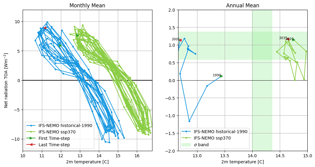
Gregory plot of IFS-NEMO historical-1990 and ssp370 simulations. The left panel represents the monthly Gregory plot, while on the right the annual Gregory plot is shown. The start and end point of the Gregory plot are indicated by the green and red arrows, respectively. In the annual Gregory plot a band representing the 2 sigma confidence interval is shown in green. This is evaluated with ERA5 data (1980-2010) for the 2m temperature and with CERES data (2000-2020) for the Net radiation TOA.
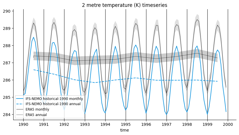
Global mean temperature time series of IFS-NEMO historical-1990 and comparison with ERA5. Both monthly and annual timeseries are shown. A 2 sigma confidence interval is evaluated for ERA5 data (1990-2020).
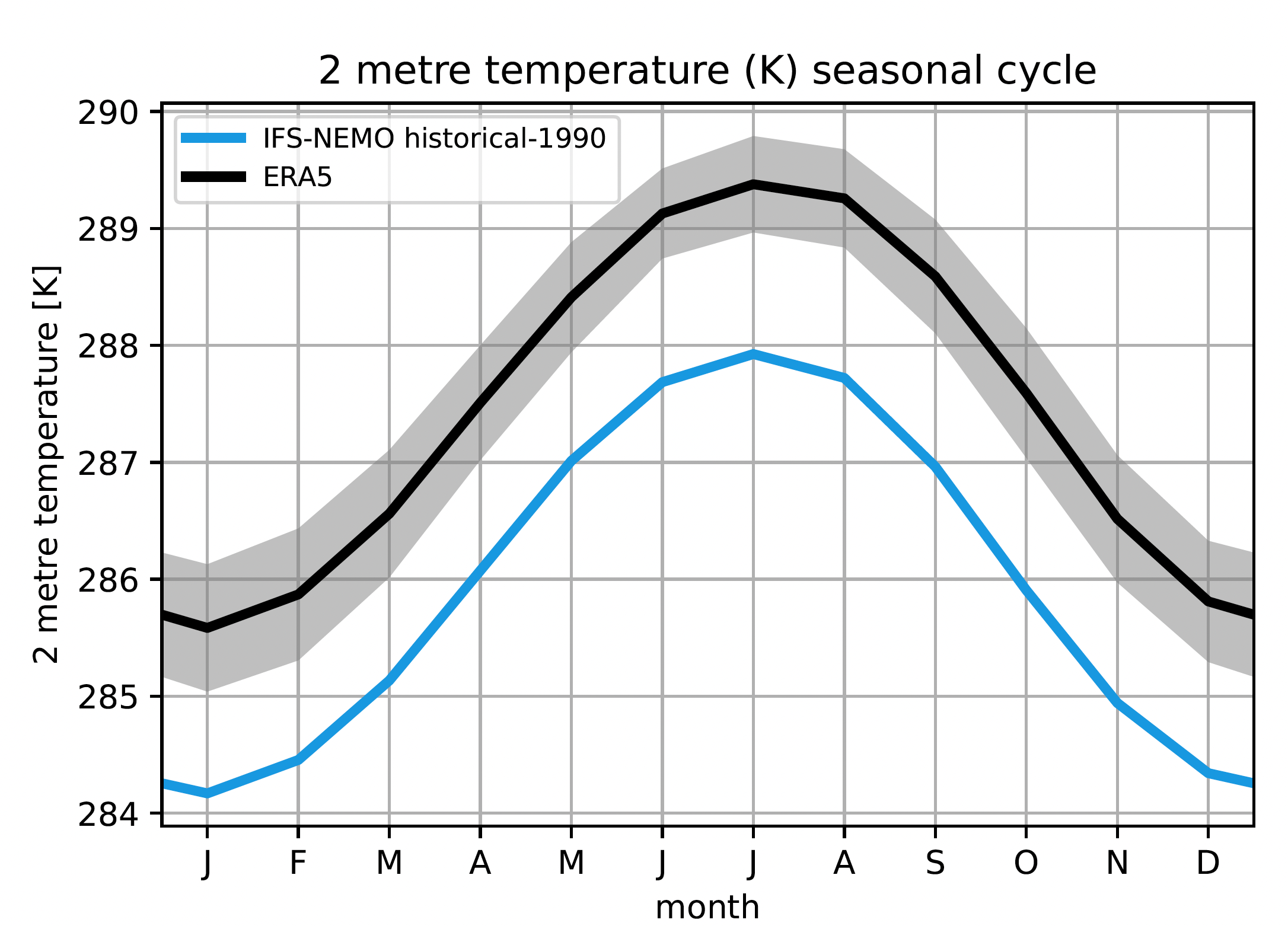
Seasonal cycle of the global mean temperature of IFS-NEMO historical-1990 and comparison with ERA5. The 2 sigma confidence interval is evaluated for ERA5 data (1990-2020).
Available demo notebooks
Notebooks are stored in diagnostics/global_time_series/notebooks
Detailed API
This section provides a detailed reference for the Application Programming Interface (API) of the timeseries diagnostic,
produced from the diagnostic function docstrings.
- class aqua.diagnostics.timeseries.GregoryPlot(catalogs=None, models=None, exps=None, sources=None, monthly=True, annual=True, regrid=None, ts_name='2t', toa_name=['tnlwrf', 'tnswrf'], ts_std_start='1980-01-01', ts_std_end='2010-12-31', toa_std_start='2001-01-01', toa_std_end='2020-12-31', ref=True, save=True, outdir='./', loglevel='WARNING', rebuild=True, filename_keys=None, save_pdf=True, save_png=True, dpi=300)
Bases:
objectGregory plot class. Retrieve data, obs reference and plot the Gregory plot. Can work with a list of models, experiments and sources.
- Parameters:
catalogs (list, opt) – List of catalogs to search for the data.
models (list) – List of model IDs.
exps (list) – List of experiment IDs.
sources (list) – List of source IDs.
monthly (bool) – If True, plot monthly data. Default is True.
annual (bool) – If True, plot annual data. Default is True.
regrid (str) – Optional regrid resolution. Default is None.
ts (str) – variable name for 2m temperature, default is ‘2t’.
toa (list) – list of variable names for net radiation at TOA, default is [‘tnlwrf’, ‘tnswrf’].
ts_std_start (str) – Start date for standard deviation calculation for 2m temperature. Default is ‘1980-01-01’.
ts_std_end (str) – End date for standard deviation calculation for 2m temperature. Default is ‘2010-12-31’.
toa_std_start (str) – Start date for standard deviation calculation for net radiation at TOA. Default is ‘2001-01-01’.
toa_std_end (str) – End date for standard deviation calculation for net radiation at TOA. Default is ‘2020-12-31’.
ref (bool) – If True, reference data is plotted. Default is True. Reference data are ERA5 for 2m temperature and CERES for net radiation at TOA.
save (bool) – If True, save the figure. Default is True.
outdir (str) – Output directory. Default is ‘./’.
loglevel (str) – Logging level. Default is WARNING.
rebuild (bool, optional) – If True, overwrite the existing files. If False, do not overwrite. Default is True.
filename_keys (list, optional) – List of keys to keep in the filename. Default is None, which includes all keys (see OutputNamer class).
save_pdf (bool) – If True, save the figure as a PDF. Default is True.
save_png (bool) – If True, save the figure as a PNG. Default is True.
dpi (int, optional) – Dots per inch (DPI) for saving figures. Default is 300.
- cleanup()
Clean up
- plot()
Plot the Gregory plot.
- retrieve_data()
Retrieve data from the given models, experiments and sources.
- retrieve_ref()
Retrieve reference data.
- run()
Retrieve ref, retrieve data and plot
- save_image(fig)
Save the figure to an image file (PDF/PNG).
- Parameters:
fig (matplotlib.figure.Figure) – Figure to save.
- save_netcdf()
Save the data to a netCDF file.
- class aqua.diagnostics.timeseries.SeasonalCycle(var=None, formula=False, catalogs=None, models=None, exps=None, sources=None, regrid=None, plot_ref=True, plot_ref_kw={'catalog': 'obs', 'exp': 'era5', 'model': 'ERA5', 'source': 'monthly'}, startdate=None, enddate=None, std_startdate=None, std_enddate=None, plot_kw={'ylim': {}}, save=True, outdir='./', longname=None, units=None, lon_limits=None, lat_limits=None, loglevel='WARNING', rebuild=None, filename_keys=None, save_pdf=True, save_png=True, dpi=300)
Bases:
TimeseriesClass to extract the seasonal cycle of a variable from a time series.
Initialize the class.
- Parameters:
var – the variable to extract the seasonal cycle
formula – if True a formula is evaluated from the variable string.
catalogs (list or str, opt) – the catalogs to search for the data
models – the list of models to analyze
exps – the list of experiments to analyze
sources – the list of sources to analyze
regrid – the regridding resolution. If None or False, no regridding is performed.
plot_ref – if True, plot the reference seasonal cycle. Default is True.
plot_ref_kw – the keyword arguments to pass to the reference plot. Default is {‘model’: ‘ERA5’, ‘exp’: ‘era5’, ‘source’: ‘monthly’}
startdate – the start date of the time series
enddate – the end date of the time series
std_startdate – the start date to evaluate the standard deviation
std_enddate – the end date to evaluate the standard deviation
plot_kw – the keyword arguments to pass to the plot
save – if True, save the figure. Default is True.
outdir – the output directory
longname – the long name of the variable. Override the attribute in the data file.
units – the units of the variable. Override the attribute in the data file.
lon_limits (list) – Longitude limits of the area to evaluate. Default is None.
lat_limits (list) – Latitude limits of the area to evaluate. Default is None.
loglevel – the logging level. Default is ‘WARNING’.
rebuild (bool, optional) – If True, overwrite the existing files. If False, do not overwrite. Default is True.
filename_keys (list, optional) – List of keys to keep in the filename. Default is None, which includes all keys (see OutputNamer class).
save_pdf (bool) – If True, save the figure as a PDF. Default is True.
save_png (bool) – If True, save the figure as a PNG. Default is True.
dpi (int, optional) – Dots per inch (DPI) for saving figures. Default is 300.
- cleanup()
Clean up the data.
- plot()
Plot the seasonal cycle.
- retrieve_ref()
Retrieve the reference data. Overwrite the method in the parent class.
- run()
Run the seasonal cycle extraction.
- save_seasonal_image(fig, ref_label)
Save the figure to an image file (PDF/PNG).
- Parameters:
fig (matplotlib.figure.Figure) – Figure to save
ref_label (str) – Label for the reference data
- save_seasonal_netcdf()
Save the seasonal cycle to a NetCDF file.
- seasonal_cycle()
Extract the seasonal cycle.
- class aqua.diagnostics.timeseries.Timeseries(var=None, formula=False, catalogs=None, models=None, exps=None, sources=None, monthly=True, annual=True, regrid=None, plot_ref=True, plot_ref_kw={'catalog': 'obs', 'exp': 'era5', 'model': 'ERA5', 'source': 'monthly'}, startdate=None, enddate=None, monthly_std=True, annual_std=True, std_startdate=None, std_enddate=None, plot_kw={'ylim': {}}, longname=None, units=None, extend=True, region=None, lon_limits=None, lat_limits=None, save=True, outdir='./', loglevel='WARNING', rebuild=None, filename_keys=None, save_pdf=True, save_png=True, dpi=300)
Bases:
objectPlot a time series of the global mean value of a given variable. By default monthly and annual time series are plotted, the annual mean is plotted as dashed line and reference data is included, ERA5 by default, with the option to plot the standard deviation as uncertainty quantification. A model, exp, source string or list of strings can be passed. If a list is passed, the time series will be plotted for each combination of model, exp and source.
- Parameters:
var (str) – Variable name.
formula (bool) – (Optional) If True, try to derive the variable from other variables. Default is False.
catalogs (list or str) – Catalog IDs.
models (list or str) – Model IDs.
exps (list or str) – Experiment IDs.
sources (list or str) – Source IDs.
regrid (str) – Optional regrid resolution. Default is None.
plot_ref (bool) – Include reference data. Default is True.
plot_ref_kw (dict) – Keyword arguments passed to get_reference_timeseries.
startdate (str) – Start date. Default is None.
enddate (str) – End date. Default is None.
annual (bool) – Plot annual mean. Default is True.
monthly_std (bool) – Plot monthly standard deviation. Default is True.
annual_std (bool) – Plot annual standard deviation. Default is True.
std_startdate (str) – Start date for standard deviation. Default is “1991-01-01”.
std_enddate (str) – End date for standard deviation. Default is “2020-12-31”.
plot_kw (dict) – Additional keyword arguments passed to the plotting function.
longname (str) – Long name of the variable. Default is None and logname attribute is used.
units (str) – Units of the variable. Default is None and units attribute is used.
extend (bool) – Extend the reference range. Default is True.
lon_limits (list) – Longitude limits of the area to evaluate. Default is None.
lat_limits (list) – Latitude limits of the area to evaluate. Default is None.
save (bool) – Save the figure. Default is True.
outdir (str) – Output directory. Default is “./”.
loglevel (str) – Log level. Default is “WARNING”.
rebuild (bool, optional) – If True, overwrite the existing files. If False, do not overwrite. Default is True.
filename_keys (list, optional) – List of keys to keep in the filename. Default is None, which includes all keys (see OutputNamer class).
save_pdf (bool) – If True, save the figure as a PDF. Default is True.
save_png (bool) – If True, save the figure as a PNG. Default is True.
dpi (int, optional) – Dots per inch (DPI) for saving figures. Default is 300.
- check_ref_range()
If the reference data don’t cover the same range as the model data, a seasonal cycle or a band of the reference data is added to the plot.
- cleanup()
Clean up
- plot()
Call an external function using the data to plot
- retrieve_data()
Retrieve data from the list and store them in a list of xarray.DataArray
- retrieve_ref(extend=True)
Retrieve reference data If the reference data don’t cover the same range as the model data, a seasonal cycle or a band of the reference data is added to the plot.
- Parameters:
extend (bool) – Extend the reference range. Default is True.
- run()
Retrieve ref, retrieve data and plot
- save_image(fig, ref_label)
Save the figure to image files (PDF/PNG). :param fig: Figure to save. :type fig: matplotlib.figure.Figure :param ref_label: Label for the reference data. :type ref_label: str
- save_netcdf()
Save the data to a netcdf file. Every model-exp-source combination is saved in a separate file. Reference data is saved in a separate file. Std data is saved in a separate file.