Teleconnections diagnostic
This package provides a diagnostic for teleconnection evaluation and comparison with ERA5 reanalysis. This is done with the computation of the teleceonnection indices and of the regression and correlation between the teleconnection index and the variable used to compute the teleconnection index.
Description
The diagnostic is based on the computation of the regression or correlation between the time series of the teleconnection index and the time series of the variable used to compute the teleconnection index. Teleconnections available:
NAO
ENSO
MJO
See Available demo notebooks for detailed examples of the usage of the diagnostic. More diagnostics or functionalities will be added in the future.
Structure
The teleconnections diagnostic is a package with a class structure.
The core of the diagnostic is in the tc_class.py file, containing the Teleconnections class.
All the source code is available in the src/aqua_diagnostics/teleconnections folder.
The source code is organized in the following way:
tc_class.pycontains the class that is used to run the diagnostic.index.pycontains functions for the direct evaluation of teleconnection indices.tc_statistics.pycontains functions for the regression and correlation analysis.bootstrap.pycontains functions for the bootstrap evaluation for concordance maps of regression and correlation.mjo.pycontains functions for the evaluation of the MJO teleconnections. This is still under development.plotsfolder contains functions for the visualization of time series and maps for teleconnection diagnostic. Part of the graphical functions are part of the AQUA framework.toolsfolder contains generic functions that may be useful to the whole diagnostic.cdo_testing.pycontains function evaluating teleconnections with cdo bindings, in order to test the python libraries.
Configuration files are available in the config/diagnostics/teleconnections folder.
Different interfaces can be used to run the diagnostic, in the context of the Destination Earth Climate DT project the interface file
is teleconnections_destine.yaml and it is used as default.
An argument interface is available in the Teleconnections class to change the interface.
It can be also customized to add new teleconnections or to change the default parameters of the diagnostic.
Notebooks are available in the notebooks/diagnostics/teleconnections folder, with detailed examples of the usage of the diagnostic.
They are organized in the following way:
NAO.ipynb contains an example of the usage of the diagnostic for the NAO index with ERA5 reanalysis.
ENSO.ipynb contains an example of the usage of the diagnostic for the ENSO index with ERA5 reanalysis.
concordance_map.ipynb contains an example of bootstrap evaluation for concordance maps of regression and correlation.
MJO.ipynb contains an example of the usage of the diagnostic for the MJO Hovmoeller plots.
A command line interface is available as cli_teleconnectios.py file in the source folder.
Tests are available in the AQUA/tests/teleconnections folder.
They make use of the pytest library and of the functions available in the cdo_testing.py library file.
Basic teleconnections diagnostic usage
The basic usage of the teleconnections diagnostic is to create an instance of the Teleconnections class and run the diagnostic.
This can be simply done with the following code:
from aqua.diagnostics import Teleconnection

tc = Teleconnection(catalog='climatedt-phase1', model='ICON', exp='ssp370', source='lra-r100-monthly', telecname='NAO')
tc.run()
This will run the diagnostic for the NAO teleconnection with the ICON model, ssp370 experiment and lra-r100-monthly source. netCDF and pdf files will be saved in the default output directory, regression and correlation maps will be saved as images and computed with the same variable of the index evaluation.
Command line interface
A command line interface is available.
cli_teleconnections.py is used to run the diagnostic from the command line.
It can analyze multiple models, exps, sources and reference datasets at the same time.
It provides a configuration file (one for the atmospheric NAO and one for the oceanic ENSO teleconnections)
to customize the details of the diagnostic.
Basic usage
Basic usage of the CLI is:
python cli_teleconnections.py
This will run the diagnostic with the default configuration file and the default model, experiment and source. It will not not compare the models with the reference dataset.
Note
The CLI is available only for ENSO and NAO teleconnections at the moment.
CLI options
The CLI accepts the following arguments:
--catalog: the catalog to analyze.--model: the model to analyze.--exp: the experiment to analyze.--source: the source to analyze.--ref: activate the reference run.-cor--config: path to the configuration file.--interface: path to the interface file.--outputdir: path to the output folder.-nor--nworkers: number of dask workers for parallel computation.-dor--dry: dry run, no files are written.-lor--loglevel: log level for the logger. Default is WARNING.--cluster: run the diagnostic on a dask cluster already existing (used by aqua-analysis).
Configuration file structure
The configuration file is a YAML file that contains the following information:
teleconnections: a block that contains the list of teleconnections to analyze. If not present, by default every teleconnection is skipped.interface: the interface file to use. Default isteleconnections_destine.yaml.models: a list of models to analyse. Here extra reader keyword can be added (e.g.regrid: 'r100',freq: 'M'). By default we assume that data are monthly and regridded to 1x1 deg resolution.reference: a block that contains the reference dataset to compare the models with. If not present, ERA5 is used as default.outputdir: the directory where the output files will be savedconfigdir: the directory where the configuration files are saved, if not present the default directory inside AQUA is used.NAOorENSO: a block that contains the parameters for the NAO or ENSO teleconnection analysis. By default NAO is evaluated for DJF and JJA, while ENSO for the full year, both with a 3 months rolling window over the original data.
Bootstrap CLI
A command line interface for bootstrap evaluation is available.
cli_bootstrap.py is used to run the bootstrap evaluation for concordance maps of regression and correlation from the command line.
This is not included in any automatic run of the diagnostic because it is a time-consuming process.
The CLI accepts the same arguments and configuration files as the basic CLI.
It produces only the netCDF files needed to plot the concordance maps, that needs to be generated in a second moment in a notebook.
You can see the example notebook concordance_map.ipynb for more details.
Input variables
The diagnostic requires the following input variables with the DestinE naming convention:
msl: (Mean sea level pressure, paramid 151) for NAOavg_tos: (Time-mean sea surface temperature, paramid 263101) for ENSOmtntrf: (Mean top net thermal radiation flux, paramid 172179) for MJO
The diagnostic can be run on any dataset that provides these variables.
It is possible to evaluate regression maps and correlation maps with a teleconnection index and a different variable.
In this case, an additional variable is needed as input.
It is also possible to use different variables if variables are missing
(e.g. for the ENSO index, the skin temperature can be used as input and have an estimate even if avg_tos is missing).
Output
The diagnostic produces the following output:
NAO: North Atlantic Oscillation index, regression and correlation maps.
ENSO: El Niño Southern Oscillation index, regression and correlation maps.
MJO: Madden-Julian Oscillation Hovmoeller plots of the Mean top net thermal radiation flux variable. A more detailed analysis is still under development.
All these outputs can be stored both as images (pdf format) and as netCDF files. If a reference dataset is provided, the automatic maps consist of contour lines for the model regression map and filled contour map for the difference between the model and the reference regression map.
Example plot
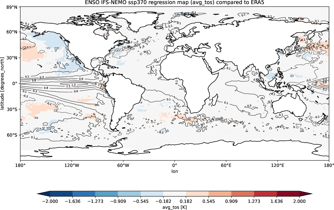
ENSO IFS-NEMO ssp370 regression map (avg_tos) compared to ERA5. The contour lines are the model regression map and the filled contour map is the difference between the model and the reference regression map (ERA5).
Available demo notebooks
Detailed API
This section provides a detailed reference for the Application Programming Interface (API) of the Teleconnections diagnostic, produced from the diagnostic function docstrings.
Teleconnections module
- class aqua.diagnostics.teleconnections.Teleconnection(model: str, exp: str, source: str, telecname: str, catalog=None, configdir=None, aquaconfigdir=None, interface='teleconnections-destine', regrid=None, freq=None, save_pdf=False, save_png=False, save_netcdf=False, outputdir='./', startdate=None, enddate=None, months_window: int = 3, loglevel: str = 'WARNING', filename_keys: list = None, rebuild: bool = True, dpi=None)
Bases:
objectClass for teleconnection objects.
- Parameters:
model (str) – Model name.
exp (str) – Experiment name.
source (str) – Source name.
telecname (str) – Teleconnection name. See documentation for available teleconnections.
catalog (str, optional) – Name of the catalog that contains the data
configdir (str, optional) – Path to diagnostics configuration folder.
aquaconfigdir (str, optional) – Path to AQUA configuration folder.
interface (str, optional) – Interface filename. Defaults to ‘teleconnections-destine’.
regrid (str, optional) – Regridding resolution. Defaults to None.
freq (str, optional) – Frequency of the data. Defaults to None.
save_pdf (bool, optional) – Save PDF if True. Defaults to False.
save_png (bool, optional) – Save PNG if True. Defaults to False.
save_netcdf (bool, optional) – Save netCDF if True. Defaults to False.
outputdir (str, optional) – Output directory for files. If None, the current directory is used.
startdate (str, optional) – Start date for the data. Format: YYYY-MM-DD. Defaults to None.
enddate (str, optional) – End date for the data. Format: YYYY-MM-DD. Defaults to None.
months_window (int, optional) – Months window for teleconnection index. Defaults to 3.
loglevel (str, optional) – Log level. Defaults to ‘WARNING’.
rebuild (bool, optional) – If True, overwrite the existing files. If False, do not overwrite. Default is True.
filename_keys (list, optional) – List of keys to keep in the filename. Default is None, which includes all keys.
dpi (int, optional) – Dots per inch (DPI) for saving figures. Default is None.
- Raises:
NoDataError – If the data is not available.
ValueError – If telecname is not one of the available teleconnections.
- evaluate_correlation(data=None, var=None, dim: str = 'time', season=None)
Evaluate teleconnection correlation. If var is None, the correlation is calculated between the teleconnection index and the teleconnection variable. If var is not None, the correlation is calculated between the teleconnection index and the specified variable. The correlation is returned as xarray.DataArray.
- Parameters:
data (xarray.DataArray, optional) – Data to be used for correlation. If None, the data used for the index is used.
var (str, optional) – Variable to be used for correlation. If None, the variable used for the index is used.
dim (str, optional) – Dimension to be used for correlation. Default is ‘time’.
season (str, optional) – Season to be selected. Default is None.
- Returns:
Correlation map
- Return type:
xarray.DataArray
- evaluate_index(rebuild=False, **kwargs)
Evaluate teleconnection index. The index is saved as teleconnection attribute and can be accessed with self.index.
- Parameters:
rebuild (bool, optional) – If True, the index is recalculated. Default is False.
**kwargs – Keyword arguments to be passed to the index function.
- Raises:
ValueError – If the index is not calculated correctly.
- evaluate_regression(data=None, var=None, dim: str = 'time', season=None)
Evaluate teleconnection regression. If var is None, the regression is calculated between the teleconnection index and the teleconnection variable. If var is not None, the regression is calculated between the teleconnection index and the specified variable. The regression is returned as xarray.DataArray.
- Parameters:
data (xarray.DataArray, optional) – Data to be used for regression. If None, the data used for the index is used.
var (str, optional) – Variable to be used for regression. If None, the variable used for the index is used.
dim (str, optional) – Dimension to be used for regression. Default is ‘time’.
season (str, optional) – Season to be selected. Default is None.
- Returns:
Regression map
- Return type:
xarray.DataArray
- plot_index(step=False, **kwargs)
Plot teleconnection index.
- Parameters:
step (bool, optional) – If True, plot the index with a step function (experimental)
**kwargs – Keyword arguments to be passed to the index_plot function.
- retrieve(var=None, **kwargs)
Retrieve teleconnection data with the AQUA reader. The data is saved as teleconnection attribute and can be accessed with self.data. If var is not None, the data is not saved as teleconnection attribute and can be accessed with the returned value.
- Parameters:
var (str, optional) – Variable to be retrieved. If None, the variable specified in the namelist
**kwargs – Keyword arguments to be passed to the reader.
- Returns:
Data retrieved if a variable is specified.
- Return type:
xarray.DataArray
- Raises:
NoDataError – If the data is not available.
- class aqua.diagnostics.teleconnections.TeleconnectionsConfig(configdir=None, interface='teleconnections-destine')
Bases:
objectClass to handle the configuration of the teleconnections diagnostic.
Initialize the TeleconnectionsConfig class.
- Parameters:
configdir (str, opt) – path to config directory. Default is None
interface (str, opt) – interface filename. Default is ‘teleconnections-destine’
- load_namelist()
Load diagnostic yaml file.
- Returns:
Diagnostic configuration
- Return type:
(dict)
- aqua.diagnostics.teleconnections.bootstrap_teleconnections(map: DataArray, index: DataArray, index_ref: DataArray, data_ref, n_bootstraps=1000, concordance=0.05, statistic=None, loglevel='WARNING', **eval_kwargs)
Bootstrap the regression and correlation maps.
- Parameters:
map (xr.DataArray) – Map of the dataset, can be regression or correlation
index (xr.DataArray) – Index of the dataset
index_ref (xr.DataArray) – Index of the reference dataset
data_ref (xr.DataArray) – Data of the reference dataset to perform the regression or correlation with.
n_bootstraps (int) – Number of bootstraps to perform. Default is 1000.
concordance (float) – Concordance threshold. Default is 0.5.
statistic (str) – Statistic to compute. Default is None. Available options are ‘reg’ and ‘cor’.
season (str) – Season to compute the statistic. Default is None.
loglevel (str) – Logging level. Default is ‘WARNING’.
eval_kwargs (dict) – Additional keyword arguments to pass to the evaluation function.
- Returns:
Lower percentile map xr.DataArray: Upper percentile map
- Return type:
xr.DataArray
- aqua.diagnostics.teleconnections.build_confidence_mask(map: DataArray, lower: DataArray, upper: DataArray, mask_concordance=True)
Build the confidence masks based on the lower and upper percentiles.
- Parameters:
reg (xr.DataArray) – Regression map of the dataset
lower (xr.DataArray) – Lower percentile map
upper (xr.DataArray) – Upper percentile map
mask_concordance (bool) – Whether to mask the concordance regions. Default is True.
- Returns:
Confidence mask
- Return type:
xr.DataArray
- aqua.diagnostics.teleconnections.cor_evaluation(indx, data, dim: str = 'time', season=None)
Evaluate correlation map of a teleconnection index and a DataArray field
- Parameters:
indx – teleconnection index
data – data field
dim (str,opt) – dimension along which to compute correlation. Default is ‘time’
season (str,opt) – season to be selected. Default is None
- Returns:
Correlation map
- Return type:
(xarray.DataArray)
- aqua.diagnostics.teleconnections.index_plot(indx, step=False, loglevel='WARNING', **kwargs)
Index plot together with a black line at indx=0. Values above 0 are filled in red, values below 0 are filled in blue.
- Parameters:
indx (DataArray) – Index DataArray
step (bool,opt) – enable or disable step plot, default is False
loglevel (str,opt) – log level for the logger, default is ‘WARNING’
**kwargs – additional arguments
- Kwargs:
figsize (tuple,opt): figure size, default is (11, 8.5)
title (str,opt): title for the plot
ylabel (str,opt): ylabel for the plot
ylim (tuple,opt): y-axis limits
fig (Figure,opt): Figure object
ax (Axes,opt): Axes object
- Returns:
Figure object ax (Axes): Axes object
- Return type:
fig (Figure)
- aqua.diagnostics.teleconnections.indexes_plot(indx1: DataArray, indx2: DataArray, titles: list = None, title: str = None, loglevel='WARNING', **kwargs)
Use the plot_index function to plot two indexes in two subplots.
- Parameters:
indx1 (-) – first index
indx2 (-) – second index
titles (-) – list of titles for the plots
title (-) – title for the figure
loglevel (-) – log level for the logger,
Kwargs are the same as for the index_plot function.
- aqua.diagnostics.teleconnections.maps_diffs_plot(maps=None, diffs=None, models=None, exps=None, titles=None, save=False, figsize=(11, 8.5), vmin_diff=None, vmax_diff=None, sym=True, nlevels=12, cbar_label=None, title=None, outputdir='.', filename='maps.png', loglevel='WARNING')
Plot maps (regression, correlation, etc.) A list of xarray.DataArray objects is expected and a map is plotted for each of them
- Parameters:
maps (list) – list of xarray.DataArray objects
diffs (list) – list of xarray.DataArray objects
models (list) – list of models
exps (list) – list of experiments
titles (list, opt) – list of titles for each map overrides models and exps standard titles
save (bool, opt) – save the figure
figsize (tuple,opt) – figure size, default is (11, 8.5)
vmin_diff (float,opt) – min value for the colorbar of the differences
vimax_diff (float,opt) – max value for the colorbar of the differences
nlevels (int,opt) – number of levels for the colorbar, default is 12
cbar_label (str,opt) – label for the colorbar
outputdir (str,opt) – output directory for the figure, default is ‘.’ (current directory)
filename (str,opt) – filename for the figure, default is ‘map.png’
loglevel (str,opt) – log level for the logger, default is ‘WARNING’
- aqua.diagnostics.teleconnections.mjo_hovmoller(data=None, var: str = None, loglevel: str = 'WARNING', telecname: str = 'MJO', namelist: dict = None, day_window: int = None, flip_sign: bool = False, **kwargs) DataArray
Prepare the data for a MJO Hovmoller plot.
- Parameters:
data – (xr.DataArray or xr.Dataset): Data to be used in the Hovmoller plot.
var (str, opt) – Name of the variable to be used in the Hovmoller plot. It is only required if data is a dataset. If not provided, it will be extracted from the namelist
loglevel (str) – Log level to be used. Default is “WARNING”.
telecname (str) – Name of the teleconnection to be evaluated. Default is “MJO”.
namelist (dict) – Namelist with the teleconnection informations.
day_window (int) – Number of days to be used in the smoothing window. Default is not performed.
flip_sign (bool) – If True, it will flip the sign of the variable. Will be extracted from the namelist if not provided. Default is False.
- KwArgs:
configdir (str): Path to the configuration directory.
- Returns:
DataArray with the data to be used in the Hovmoller plot.
- Return type:
xr.DataArray
- aqua.diagnostics.teleconnections.reg_evaluation(indx, data, dim: str = 'time', season=None)
Evaluate regression map of a teleconnection index and a DataArray field
- Parameters:
indx – teleconnection index
data – data field
dim (str,opt) – dimension along which to compute regression. Default is ‘time’
season (str,opt) – season to be selected. Default is None
- Returns:
Regression map
- Return type:
(xarray.DataArray)
- aqua.diagnostics.teleconnections.regional_mean_anomalies(field, namelist, telecname, months_window=3, loglevel='WARNING')
Evaluate regional field mean anomalies for a teleconnection. Data must be monthly gridded data.
- Parameters:
field (xarray.DataArray) – field over which evaluate the index
namelist – teleconnection yaml infos
telecname (str) – name of the teleconnection to be evaluated
months_window (int, opt) – months for rolling average, default is 3
loglevel (str, opt) – log level, default is WARNING
- Returns:
regional field mean anomalies
- Return type:
(xarray.DataArray)
- aqua.diagnostics.teleconnections.regional_mean_index(field, namelist, telecname, months_window=3, loglevel='WARNING')
Evaluate regional field mean for a teleconnection. Data must be monthly gridded data.
- Parameters:
field (xarray.DataArray) – field over which evaluate the index
namelist – teleconnection yaml infos
telecname (str) – name of the teleconnection to be evaluated
months_window (int, opt) – months for rolling average, default is 3
loglevel (str, opt) – log level, default is WARNING
- Returns:
regional field mean
- Return type:
(xarray.DataArray)
- aqua.diagnostics.teleconnections.station_based_index(field: DataArray, namelist: dict, telecname='NAO', months_window=3, loglevel='WARNING')
Evaluate station based index for a teleconnection. Field data must be monthly gridded data.
- Parameters:
field (xr.DataArray) – field over which evaluate the index
namelist (dict) – teleconnection yaml infos
telecname (str, opt) – name of the teleconnection to be evaluated Default is NAO
months_window (int, opt) – months for rolling average, default is 3
loglevel (str, opt) – log level, default is WARNING
- Returns:
standardized station based index
- Return type:
(xarray.DataArray)
- aqua.diagnostics.teleconnections.wgt_area_mean(indat, latN: float, latS: float, lonW: float, lonE: float, box_brd=True, loglevel='WARNING')
Evaluate the weighted mean of a quantity on a custom surface.
- Parameters:
indat (xarray.DataArray) – input data to be averaged
latN (float) – North latitude
latS (float) – South latitude
lonW (float) – West longitude
lonE (float) – Est longitude
box_brd (bool,opt) – choose if coordinates are comprised or not. Default is True
loglevel (str, opt) – log level, default is WARNING
- Returns:
average of input data on a custom surface
- Return type:
(xarray.DataArray)