Sea ice

Description

The Sea Ice diagnostic is a set of tools to compute and plot time series, seasonal cycles and 2D spatial maps of sea ice metrics. The diagnostic supports analysis of sea ice extent, volume, fraction, and thickness. Time series and seasonal cycles can be computed over a specific region of the Northern or Southern Hemisphere. Default regions are the Arctic and the Antarctic regions, but it is possible to select other regions and custom regions can be defined in the configuration file.

Classes

There is one class that process and analyse the sea ice data, allowing to save the result as NetCDF files:

SeaIce: a class that computes the sea ice extent, volume, fraction, and thickness metrics. The class handles data retrieval, regional selection, integration, and statistical analysis internally for a single model or reference data. It supports time series analysis and seasonal cycle computation with optional standard deviation calculations.
- The methods supported for time series analysis which computes the integrated values over specified regions are:
  - extent: computes the area of ocean cells with at least 15% sea ice concentration (the threshold can be tuned in the configuration file).
  - volume: computes the integrated sea ice thickness.
- The methods supported for 2D spatial analysis, which computes the 2D monthly climatology maps over specified regions are:
  - fraction: produces the 2D monthly climatology maps of sea ice fraction (0-1).
  - thickness: produces the 2D monthly climatology maps of sea ice thickness (meters).

There are other two classes to produce the plots, which support a comparison between multiple models against a reference dataset. These classes can accept a xarray.DataArray, a xarray.Dataset, or a list of xarray.Dataset with a collection of sea ice variables defined per region and calculation method.

PlotSeaIce: a class that produces time series and seasonal cycle plots.
Plot2DSeaIce: a class that produces the plots for the 2D spatial maps and biases for climatological maps over the months.

Note

The extent and volume methods produce time series data, while fraction and thickness methods is associated to 2D spatial maps.

File structure

The diagnostic is located in the src/aqua_diagnostics/seaice directory, which contains both the source code and the command line interface (CLI) script cli_seaice.py.
The default configuration file is located in config/diagnostics/seaice/config_seaice.yaml.
The regional definitions are defined in config/diagnostics/seaice/definitions/regions.yaml.
Notebooks are available in notebooks/diagnostics/seaice directory and contain examples of how to use the diagnostic.

Input variables and datasets

The classes support the following variables, although the Fixer class can convert the acceptable different variable names into the following accepted variables:

siconc (sea ice concentration, GRIB parameter id 31)
sithick (sea ice thickness, GRIB parameter id 32)
sivol (sea ice volume, GRIB parameter id 33)

The diagnostic supports comparison with reference datasets, with OSI-SAF being the default observational reference for sea ice concentration. Custom reference datasets can be configured through the configuration file.

Basic usage

The basic usage of this diagnostic is explained with a working example in the notebook provided in the notebooks/diagnostics/seaice directory. A basic structure of the analysis is the following:

For Time Series Analysis:

from aqua.diagnostics import SeaIce, PlotSeaIce

# Compute sea ice extent (time series calculation)
si = SeaIce(model='IFS-NEMO', exp='historical-1990', source='lra-r100-monthly', loglevel="DEBUG")
result = si.compute_seaice(method='extent', var='siconc')

# Plot time series
psi = PlotSeaIce(monthly_models=result, loglevel='DEBUG')
psi.plot_seaice(plot_type='timeseries', save_pdf=True, save_png=True)

For 2D Spatial Analysis:

from aqua.diagnostics import SeaIce, Plot2DSeaIce

# Compute sea ice fraction (2D maps calculation)
si = SeaIce(model='IFS-NEMO', exp='historical-1990', source='lra-r100-monthly', loglevel="DEBUG")
result = si.compute_seaice(method='fraction', var='siconc', stat='mean', freq='monthly')

# Plot 2D maps
psi_2d = Plot2DSeaIce(models=result, loglevel='DEBUG')
psi_2d.plot_2d_seaice(plot_type='var', method='fraction', months=[3,9],
                      projkw={'projname': 'orthographic'}, save_pdf=True, save_png=True)

Note

The user can also define the start and end date of the analysis and the reference dataset. If not specified otherwise, plots will be saved in PNG and PDF format in the current working directory.

CLI usage

The diagnostic can be run from the command line interface (CLI) by running the following command:

cd $AQUA/src/aqua_diagnostics/seaice
python cli_seaice.py --config <path_to_config_file>

Additionally, the CLI can be run with the following optional arguments:

--config, -c: Path to the configuration file. Default is config/diagnostics/seaice/config_seaice.yaml in the AQUA root directory.
--nworkers, -n: Number of workers to use for parallel processing.
--cluster: Cluster to use for parallel processing. By default a local cluster is used.
--loglevel, -l: Logging level. Default is WARNING.
--catalog: Catalog to use for the analysis. Can be defined in the config file.
--model: Model to analyse. Can be defined in the config file.
--exp: Experiment to analyse. Can be defined in the config file.
--source: Source to analyse. Can be defined in the config file.
--outputdir: Output directory for the plots.
--proj: Projection type for 2D plots. Choices are ‘orthographic’ or ‘azimuthal_equidistant’. Default is ‘orthographic’.

Config file structure

The configuration file is a YAML file that contains the details on the dataset to analyse or use as reference, the output directory and the diagnostic settings. Most of the settings are common to all the diagnostics (see Diagnostics configuration files). Here we describe only the specific settings for the sea ice diagnostic.

The sea ice configuration file is organized into several main sections

Dataset Configuration:

datasets:
  - catalog: null              # mandatory as null
    model: 'IFS-NEMO'          # mandatory
    exp: 'historical-1990'     # mandatory
    source: 'lra-r100-monthly' # mandatory
    regrid: null               # if the diagnostic supports it

Reference Datasets:

references:
  # ---- Extent in NH ----
  - &ref_osi_nh
    catalog: 'obs'             # mandatory
    model: 'OSI-SAF'           # mandatory
    exp: 'osi-450'             # mandatory
    source: 'nh-monthly'       # mandatory
    regrid: 'r100'
    domain: "nh"

The reference datasets are defined using YAML anchors (&ref_osi_nh) and can be reused across different diagnostic blocks. Each reference dataset specifies:

catalog: Data catalog identifier
model: Reference model name (e.g., OSI-SAF, PSC)
exp: Experiment identifier
source: Data source specification
regrid: Regridding target resolution
domain: Geographic domain (nh=Northern Hemisphere, sh=Southern Hemisphere)

Diagnostic Blocks:

Each diagnostic block in CLI config_seaice.yaml:

seaice_timeseries
seaice_seasonal_cycle
seaice_2d_bias

contains the following parameters such as:

seaice_timeseries:
  run: true
  methods: ["extent", "volume"]   # Methods to compute
  regions: ['arctic','antarctic'] # Regions to analyze
  startdate: '1991-01-01'         # Analysis start date
  enddate: '2000-01-01'           # Analysis end date
  calc_ref_std: true              # Calculate reference standard deviation
  ref_std_freq: 'monthly'         # Standard deviation frequency
  varname:                        # Variable mapping for each method
    extent: 'siconc'
    volume: 'sithick'
    fraction: 'siconc'
    thickness: 'sithick'

Method-specific variable mapping:

extent and fraction: Use siconc as variable name (sea ice concentration)
volume and thickness: Use sithick as variable name (sea ice thickness)

Reference dataset assignment:

Each diagnostic block includes a references section that assigns specific reference datasets to methods:

references:
  - <<: *ref_osi_nh
    use_for_method: "extent"    # Use this reference for extent analysis
    varname: "siconc"
  - <<: *ref_psc_nh
    use_for_method: "volume"    # Use this reference for volume analysis
    varname: "sithick"

2D Bias Configuration: The seaice_2d_bias block includes additional parameters for spatial analysis:

seaice_2d_bias:
  months: [3, 9]                # Months to plot (March and September)
  projections:                  # Map projection options
    orthographic:
      projname: "orthographic"
      projpars:
        central_longitude: 0.0
        central_latitude: "max_lat_signed"
    extent_regions:             # Geographic extent for each region
      Arctic: [-180, 180, 50, 90]
      Antarctic: [-180, 180, -50, -90]

projections can be tuned to the user according to the section ‘Projections and custom maps’ in Graphic tools.

Output Configuration:

output:
  outputdir: "./"               # Output directory
  rebuild: true                 # Overwrite existing files
  save_netcdf: true             # Save NetCDF files
  save_pdf: true                # Save PDF plots
  save_png: true                # Save PNG plots
  dpi: 300                      # Plot resolution

Note

The configuration file uses YAML anchors (&ref_osi_nh) and references (<<: *ref_osi_nh) to avoid duplication. This allows the same reference dataset definition to be reused across different diagnostic blocks with method-specific assignments.

CLI processing

The CLI uses separate diagnostic blocks for different types of analysis:

seaice_timeseries: for time series analysis of extent and volume
seaice_seasonal_cycle: for seasonal cycle analysis of extent and volume
seaice_2d_bias: for 2D spatial analysis of fraction and thickness biases

The input parameters can be overridden during the CLI call.

Outputs

After the analysis and processing of the data, the diagnostic can produce the following outputs:

NetCDF files: Time series, seasonal cycle or 2D spatial climatology maps saved in NetCDF format for further analysis.

All plots can be performed and then saved in both PDF and PNG formats with comprehensive metadata describing the plot:

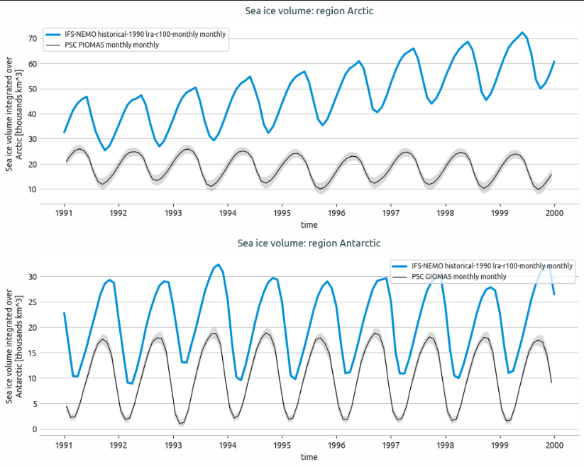
Time series plots: Monthly time series of sea ice extent and volume for specified regions.
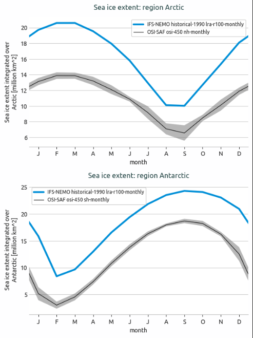
Seasonal cycle plots: Monthly climatology of sea ice metrics with optional standard deviation bands.
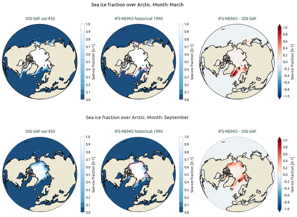
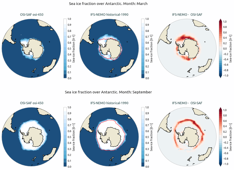
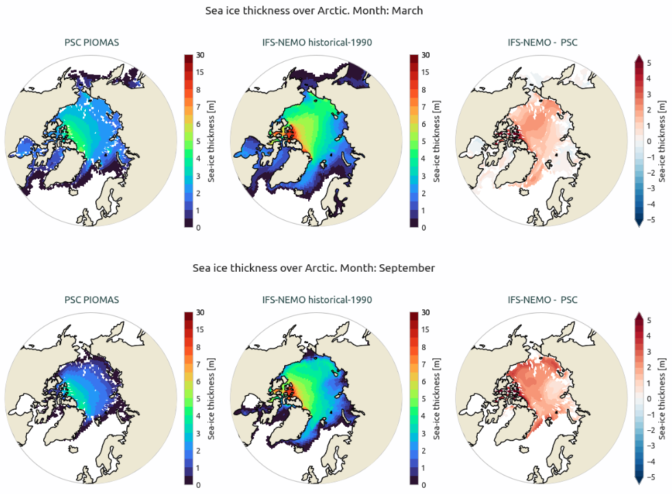
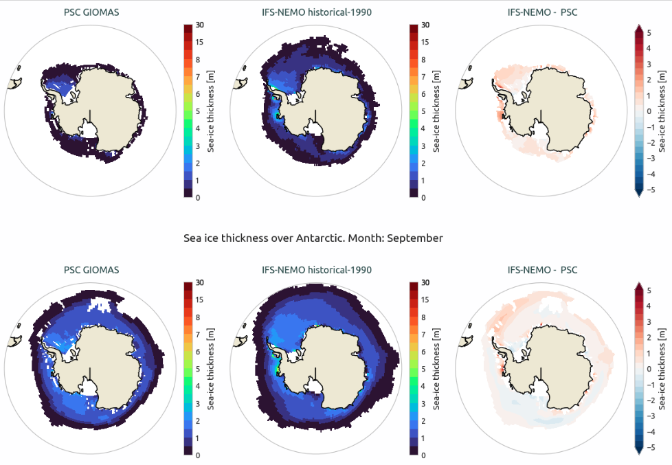
2D spatial maps: Climatological maps of sea ice fraction and thickness for specific months and regions.
Bias maps: Spatial differences between model and reference sea ice data for specific months and regions.

Example Plot(s)

../_images/seaice_ts_volume_Arctic_Antarctic.png

../_images/seaice_seasonalcycle_extent_Arctic_Antarctic.png

../_images/seaice_2d_fraction_Arctic_3-9.png

../_images/seaice_2d_fraction_Antarctic_3-9.png

../_images/seaice_2d_thickness_Arctic_3-9.png

../_images/seaice_2d_thickness_Antarctic_3-9.png

Observations (Reference data)

Default model is IFS-NEMO, experiment is historical-1990, source is lra-r100-monthly.

Details on the reference datasets, are available on the website of the Ocean and Sea Ice Satellite Application Facility (OSI-SAF) here. An updated version of the reference datasets is available in AQUA obs catalog named exp=osi-saf-aqua, which concatentes OSI-SAF osi-450-a1 (1979 - 2021) and OSI-SAF osi-430 (2022 - 2024) datasets.

Available demo notebooks

Notebooks are stored in diagnostics/seaice/notebooks

Authors and contributors

This diagnostic is maintained by Emanuele Tovazzi (@tovaz92, emanueletovazzi [at] cnr.it), member of the AQUA team. Contributions are welcome — please open an issue or a pull request. For questions or suggestions, contact the AQUA team or the maintainers.

Detailed API

This section provides a detailed reference for the Application Programming Interface (API) of the Seaice diagnostic, produced from the diagnostic function docstrings.