Timeseries
Description
The Timeseries diagnostic is a set of tools to compute and plot time series, seasonal cycles and Gregory-like plot of a given variable or formula for a given model or list of models. Time series and seasonal cycles can be computed globally or for a specific area. The three functionalities are designed to have a class which analyse a single model to produce the netCDF files and another class to produce the plots. The diagnostic can compare the model time series with a reference dataset, which is defined in the configuration file.
Classes
There are three classes to compute the netCDF files:
Timeseries: a class that computes time series of a given variable or formula for a given model or dataset. Comparison with a reference dataset is also possible. It supports hourly, daily, monthly and yearly time series and area selection. It can also compute the standard deviation of the time series.
SeasonalCycles: a class that computes the seasonal cycle of a given variable or formula for a given model or dataset. Comparison with a reference dataset is also possible. It can also compute the standard deviation of the seasonal cycle. It supports area selection.
Gregory: a class that computes the monthly and annual time series necessary for the Gregory-like plot of net radiation TOA and 2 metre temperature. It can also compute the standard deviation of the time series.
There are three other classes to produce the plots:
PlotTimeseries: a class that ingests xarrays and produces the plots for the time series. Info necessary for titles, legends and captions are deduced from the xarray attributes.
PlotSeasonalCycles: a class that ingests xarrays and produces the plots for the seasonal cycle. Info necessary for titles, legends and captions are deduced from the xarray attributes.
PlotGregory: a class that ingests xarrays and produces the Gregory-like plot. Info necessary for titles, legends and captions are deduced from the xarray attributes.
Warning
Hourly and daily plots are not available yet, while the netCDF files are produced.
File structure
The diagnostic is located in the
src/aqua_diagnostics/timeseriesdirectory, which contains both the source code and the command line interface (CLI) script.The configuration files are located in the
config/diagnostics/timeseriesdirectory and contains the default configuration for the diagnostic.Notebooks are available in the
notebooks/diagnostics/timeseriesdirectory and contain examples of how to use the diagnostic.A list of available regions is available in the
config/diagnostics/timeseries/interface/regions.yamlfile.
Input variables and datasets
By default, the diagnostic compare against the ERA5 dataset, with standard deviation calculated over the period 1990-2020. The Gregory-like plot uses the CERES dataset for the Net radiation TOA and the ERA5 dataset for the 2 metre temperature.
The necessary input variables for the diagnostic are all the variables that are needed to compute the time series, seasonal cycle choosen in the configuration file. The Gregory-like plot requires the Net radiation TOA and the 2 metre temperature.
CLI usage
The diagnostic can be run from the command line interface (CLI) by running the following command:
cd $AQUA/src/aqua_diagnostics/timeseries
python cli_timeseries.py --config <path_to_config_file>
Three configuration files are provided and run when executing the aqua-analysis (see AQUA analysis wrapper). Two configuration files are for atmospheric and oceanic timeseries and gregory plots, and the third one is for the seasonal cycles.
Additionally CLI arguments are described in the Diagnostics CLI arguments section.
Config file structure
The configuration file is a YAML file that contains the details on the dataset to analyse or use as reference, the output directory and the diagnostic settings. Most of the settings are common to all the diagnostics (see Diagnostics configuration files). Here we describe only the specific settings for the time series diagnostic.
timeseries: a block, nested in thediagnosticsblock, that contains the details required for the time series. The parameters specific to a single variable are merged with the default parameters, giving priority to the specific ones.
diagnostics:
  timeseries:
    run: true # to enable the time series
    diagnostic_name: 'atmosphere'
    variables: ['2t', 'tprate']
    formulae: ['tnlwrf+tnswrf']
    center_time: true # center the time axis of the time series
    params:
      default:
        hourly: false # Frequency to enable
        daily: false
        monthly: true
        annual: true
        std_startdate: '1990-01-01'
        std_enddate: '2020-12-31'
      tnlwrf+tnswrf:
        short_name: "net_top_radiation"
        long_name: "Net top radiation"
      tprate:
        units: 'mm/day'
        short_name: 'tprate'
        long_name: 'Total precipitation rate'
        regions: ['tropics', 'europe'] # regions to plot the time series other than global
seasonalcycle: a block, nested in thediagnosticsblock, that contains the details required for the seasonal cycle. The parameters specific to a single variable are merged with the default parameters, giving priority to the specific ones.
diagnostics:
  seasonalcycle:
    run: true # to enable the seasonal cycle
    diagnostic_name: 'atmosphere'
    variables: ['2t', 'tprate']
    center_time: true # center the time axis of the seasonal cycle
    params:
      default:
        std_startdate: '1990-01-01'
        std_enddate: '2020-12-31'
      tprate:
        units: 'mm/day'
        long_name: 'Total precipitation rate'
gregory: a block, nested in thediagnosticsblock, that contains the details required for the Gregory-like plot.
diagnostics:
  gregory:
    run: true # to enable the Gregory plot
    t2m: '2t' # variable name for the 2 metre temperature
    net_toa_name: 'tnlwrf+tnswrf' # formula or variable name for the Net radiation TOA
    monthly: true
    annual: true
    std: true
    std_startdate: '1990-01-01'
    std_enddate: '2020-12-31'
    # Gregory needs 2 datasets and do not care about the references block above
    t2m_ref: {'catalog': 'obs', 'model': 'ERA5', 'exp': 'era5', 'source': 'monthly'}
    net_toa_ref: {'catalog': 'obs', 'model': 'CERES', 'exp': 'ebaf-toa42', 'source': 'monthly'}
Output
The diagnostic produces three types of plots (see Example Plots):
A comparison of monthly and/or annual global mean time series of the model and the reference dataset.
A comparison of the seasonal cycle of the model and the reference dataset.
A Gregory-like plot of the model and the reference dataset as bands.
The timeseries, reference timeseries and standard deviation timeseries are also saved in the output directory as netCDF files.
Observations
The diagnostic uses the following reference datasets:
ERA5 as a default reference dataset for the global mean time series and seasonal cycle.
ERA5 for the 2m temperature and CERES for the Net radiation TOA in the Gregory-like plot.
Note
Multiple reference time series and seasonal cycles plot are planned for the future.
Custom reference datasets can be used.
Example Plots
A plot for each class is shown below.
All these plots can be produced by running the notebooks in the notebooks directory on LUMI HPC.
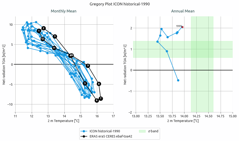
Gregory plot of ICON historical-1990 simulation.
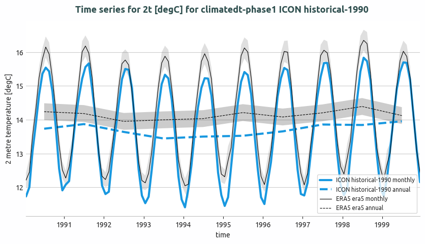
Global mean temperature time series of ICON historical-1990 and comparison with ERA5. Both monthly and annual timeseries are shown. A 2 sigma confidence interval is evaluated for ERA5 data (1990-2020).
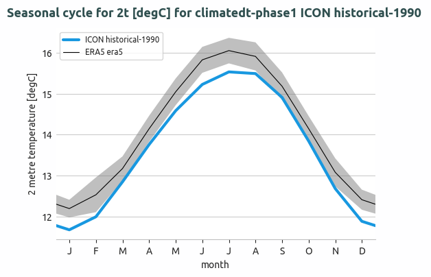
Seasonal cycle of the global mean temperature of IFS-NEMO historical-1990 and comparison with ERA5. The 2 sigma confidence interval is evaluated for ERA5 data (1990-2020).
Available demo notebooks
Notebooks are stored in the notebooks/diagnostics/timeseries directory and contain examples of how to use the diagnostic.
Detailed API
This section provides a detailed reference for the Application Programming Interface (API) of the timeseries diagnostic,
produced from the diagnostic function docstrings.